文本介绍xDeepFM的理论介绍,包括阅读论文后自己的理解
- 上篇博客参考: DeepFM
- 原始论文: xDeepFM: Combining Explicit and Implicit Feature Interactions for Recommender Systems, KDD 2018
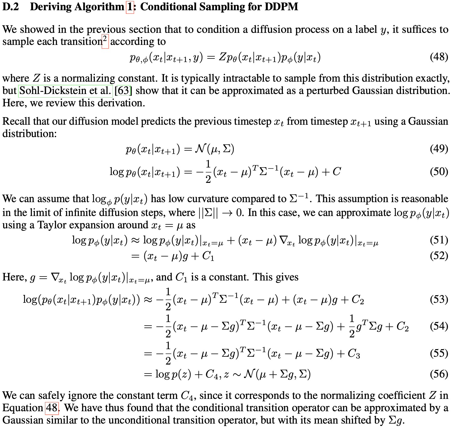
xDeepFM结构图
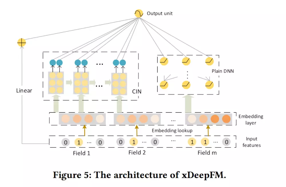
- 显然, 上图中除了 CIN 部分以外,其他跟 DeepFM 基本是相同的, 所以我们论文主要讲述 CIN 组件部分, 其他的嵌入层等可参考我之前的博客DeepFM
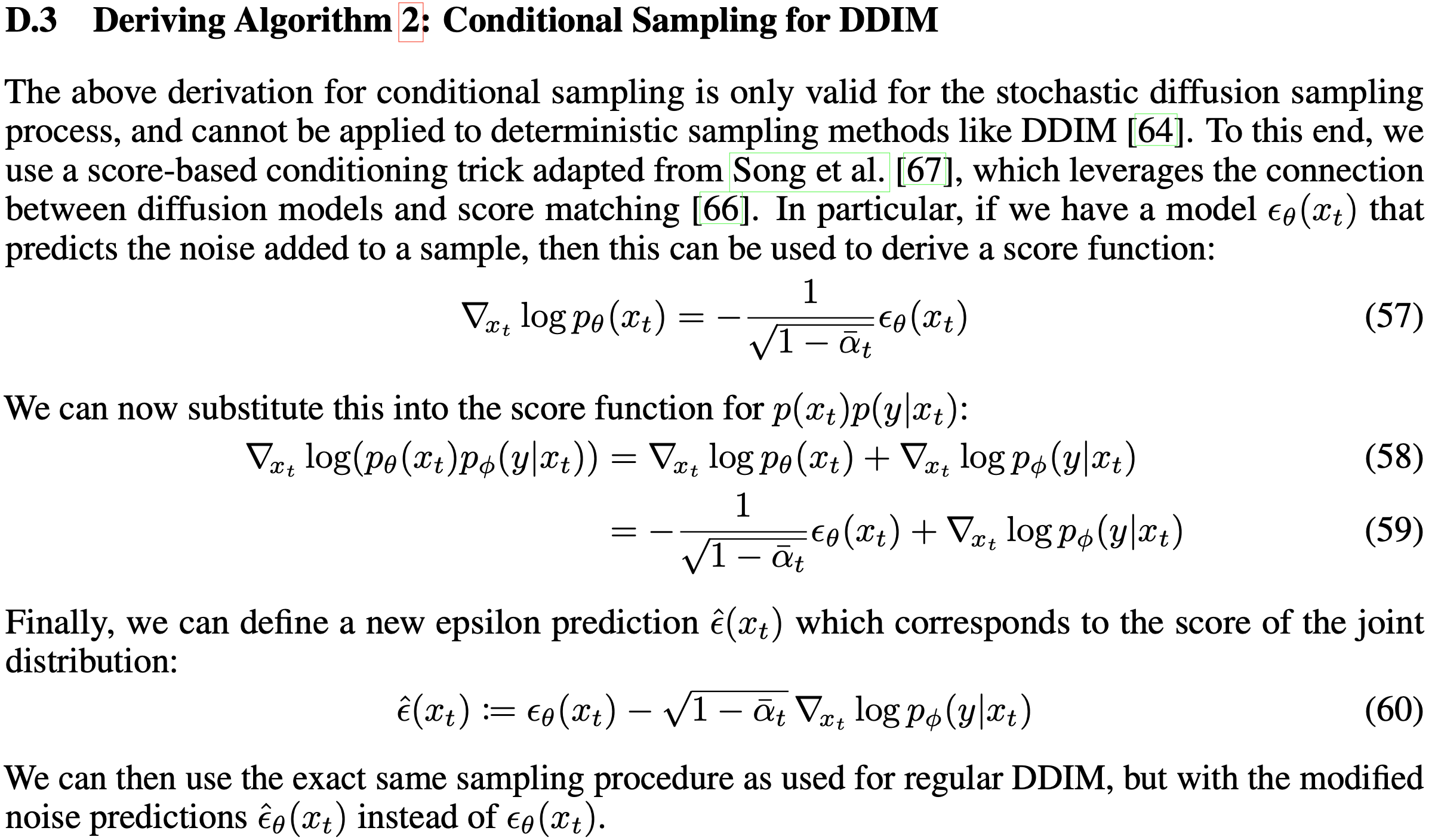
CIN组件
Compressed Interaction Network
- 论文中首先提出的就是这个CIN网络(Compressed Interaction Network)
- 结构图如下:
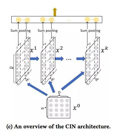
- 理解
- 每个隐藏层都与一个池化操作连接到一起
- 特征阶数与网络层数相关
- 可以与 RNN 对应着看, 当前网络层由上一个隐藏层和一个额外输入确定
- 确切的说: CIN 中当前层输入是前一层的隐藏层 + 原来的特征向量