Hexo

凡事预则立,不预则废


  • Home

  • Tags

  • Archives

  • Navigation

  • Search

DL——RectifiedFlow

  • 参考链接:
    • 原始论文:Flow Straight and Fast: Learning to Generate and Transfer Data with Rectified Flow, 202209,虽然原理很简单,但是原始论文证明比较详细,且伪代码不够清晰(包含一些数据内容),所以显得晦涩难懂

Rectified Flow 整体说明

  • Rectified Flow 是一种基于常微分方程(ODE)的生成模型,旨在通过“直线化”轨迹实现高效采样。其核心思想是通过优化一个速度场(velocity field)来最小化传输映射的误差,从而将源分布(如高斯噪声)转换为目标分布(如图像数据)
  • Rectified Flow 的训练通过优化速度场和 Reflow 技术逐步拉直轨迹,而采样则通过 ODE 求解实现高效生成。其核心贡献在于简化扩散模型的复杂推导 ,并通过直线化路径实现快速采样 ,适用于生成、迁移等多种任务

Rectified Flow 训练过程

  • Rectified Flow 的训练分为两个主要阶段:初始训练(1-Rectified Flow)和轨迹优化(Reflow)

初始训练(1-Rectified Flow)

  • 目标 :学习一个速度场 \( v(X_t, t) \),使得从源分布 \( \pi_0 \)(如高斯噪声)到目标分布 \( \pi_1 \)(如真实图像)的传输路径尽可能直线化
  • 数据配对 :随机采样 \( X_0 \sim \pi_0 \) 和 \( X_1 \sim \pi_1 \),并假设它们之间通过线性插值连接:
    $$
    X_t = t X_1 + (1-t) X_0, \quad t \in [0,1]
    $$
  • 损失函数 :最小化速度场 \( v \) 与理想直线方向 \( (X_1 - X_0) \) 的均方误差:
    $$
    \min_v \int_0^1 \mathbb{E}_{X_0, X_1} \left[ | (X_1 - X_0) - v(X_t, t) |^2 \right] dt
    $$
    • 其中 \( X_t \) 是插值点

Reflow(轨迹优化,可选,可多次执行)

  • 问题 :初始训练中 \( X_0 \) 和 \( X_1 \) 是随机配对的,导致轨迹可能交叉或弯曲,影响采样效率
  • 解决方案 :使用已训练的 1-Rectified Flow 生成新的配对数据 \( (X_0, \text{Flow}_1(X_0)) \),再训练一个新的速度场(2-Rectified Flow)。这样,轨迹会变得更直,减少交叉
  • 数学表达 :
    $$
    \min_v \int_0^1 \mathbb{E}_{X_0 \sim \pi_0, X_1 \sim \text{Flow}_1(X_0)} \left[ | (X_1 - X_0) - v(X_t, t) |^2 \right] dt
    $$
  • 迭代优化 :可以多次应用 Reflow ,逐步拉直轨迹,提高采样效率
  • 可理论证明这是 Reflow 的单调改进

采样过程

  • Rectified Flow 的采样过程通过数值求解 ODE 实现,通常使用欧拉法(Euler method)或更高阶的数值积分器

标准采样(多步)

  • 从 \( Z_0 \sim \pi_0 \) 开始,逐步计算:
    $$
    Z_{t+\Delta t} = Z_t + v(Z_t, t) \cdot \Delta t
    $$
    • 其中 \( \Delta t = 1/N \),\( N \) 是步数
    • 由于轨迹已被 Reflow 拉直,即使步数较少(如 10-20 步),也能生成高质量样本
    • 采样时 \(t = 0 \rightarrow 1\)

一步生成(蒸馏)

  • 经过 Reflow 后,轨迹足够直,可以尝试一步生成:
    $$
    Z_1 = Z_0 + v(Z_0, 0)
    $$
    • 这一步相当于直接预测 \( X_1 - X_0 \),但需要高质量的 Reflow 训练

Rectified Flow 对比传统 Diffusion 模型

  • Rectified Flow 采样更高效 :相比传统扩散模型(如 DDPM),Rectified Flow 的直线化轨迹允许更少的采样步数,甚至一步生成
  • Rectified Flow 应用范围更广 :Rectified Flow 的本质是拟合一个分布到另一个分布,不仅可用于生成模型(噪声到图像),还可用于域迁移(如猫脸到人脸)
  • 其他说明 :使用 Reflow 能不断降低传输代价,使轨迹越来越直,可理论证明这是 Reflow 的单调改进
  • 采样时 \(t\) 的取值不同,但都表示从噪声到真实图片的生成过程:
    • Diffusion Model 是 \(t = T \rightarrow 1\),逐渐减小
    • Rectified Flow 是 \(t = 0 \rightarrow 1\),逐渐增大,详情见附录代码示例输出结果
      • 注:这是由于训练时使用的混合值方式不同造成的,微改一下混合方式,\(t\) 的取值也可以逐渐变小

Rectified Flow 应用场景

  • Stable Diffusion 3 采用了 Rectified Flow 的改进版本,结合 Transformer 架构,在高分辨率文本到图像生成中表现优异

Rectified Flow 的证明过程

  • 待补充

附录:Rectified Flow 代码示例

  • 一个简单的 Rectified Flow 训练和采样代码示例

    1
    2
    3
    4
    5
    6
    7
    8
    9
    10
    11
    12
    13
    14
    15
    16
    17
    18
    19
    20
    21
    22
    23
    24
    25
    26
    27
    28
    29
    30
    31
    32
    33
    34
    35
    36
    37
    38
    39
    40
    41
    42
    43
    44
    45
    46
    47
    48
    49
    50
    51
    52
    53
    54
    55
    56
    57
    58
    59
    60
    61
    62
    63
    64
    65
    66
    67
    68
    69
    70
    71
    72
    73
    74
    75
    76
    77
    78
    79
    80
    81
    82
    83
    84
    85
    86
    87
    88
    89
    90
    91
    92
    93
    94
    95
    96
    97
    98
    99
    100
    101
    102
    103
    104
    105
    106
    107
    108
    109
    110
    111
    112
    113
    114
    115
    116
    117
    118
    119
    120
    121
    122
    123
    124
    125
    126
    127
    128
    129
    130
    131
    132
    133
    134
    135
    136
    137
    138
    139
    140
    141
    142
    143
    144
    145
    146
    147
    148
    149
    150
    151
    152
    153
    154
    155
    156
    157
    158
    159
    160
    161
    162
    163
    import torch
    import torch.nn as nn
    import torch.optim as optim
    import numpy as np
    import matplotlib.pyplot as plt
    from torch.utils.data import Dataset, DataLoader
    from sklearn.datasets import make_moons

    # 可兼容旧版本PyTorch的SiLU实现,新版本中直接使用 nn.SiLU即可
    if hasattr(nn, 'SiLU'):
    SiLU = nn.SiLU
    else:
    class SiLU(nn.Module):
    def forward(self, x):
    return x * torch.sigmoid(x)

    # 设置随机种子
    torch.manual_seed(42)
    np.random.seed(42)

    # 超参数
    batch_size = 512
    lr = 1e-3
    epochs = 2000
    num_samples = 10000 # 生成的数据点数量
    dim = 2 # 数据维度

    # 创建一个简单的 2D 数据集 (两个半圆月亮)
    class MoonsDataset(Dataset):
    def __init__(self, n_samples):
    X, _ = make_moons(n_samples=n_samples, noise=0.05)
    self.x = torch.tensor(X, dtype=torch.float32)

    def __len__(self):
    return len(self.x)

    def __getitem__(self, idx):
    return torch.FloatTensor(self.x[idx])


    # 创建一个简单的 2D 数据集 (两个半圆拼凑成一个圆形)
    class CircleDataset(Dataset):
    def __init__(self, num_samples):
    theta = np.random.uniform(0, np.pi, num_samples)
    self.x = np.stack([
    np.concatenate([np.cos(theta), np.cos(theta)]),
    np.concatenate([np.sin(theta), -np.sin(theta)])
    ], axis=1)
    self.x = self.x + 0.1 * np.random.randn(*self.x.shape) # 添加噪声

    def __len__(self):
    return len(self.x)

    def __getitem__(self, idx):
    return torch.FloatTensor(self.x[idx])

    # 定义一个简单的 MLP 作为流模型
    class FlowModel(nn.Module):
    def __init__(self, dim=2, hidden_dim=128):
    super().__init__()
    self.net = nn.Sequential(
    nn.Linear(dim + 1, hidden_dim), # +1 对应时间 t
    SiLU(),
    nn.Linear(hidden_dim, hidden_dim),
    SiLU(),
    nn.Linear(hidden_dim, dim)
    )

    def forward(self, x, t):
    # x: (batch_size, dim), t: (batch_size, 1)
    t = t.view(-1, 1)
    inputs = torch.cat([x, t], dim=1)
    return self.net(inputs)

    # 训练函数
    def train(model, dataloader, optimizer, epochs):
    model.train()
    loss_history = []
    for epoch in range(epochs):
    total_loss = 0
    for x1 in dataloader:
    x1 = x1.to(device) # 真实数据 x1
    t = torch.rand(x1.size(0), device=device).view(-1,1) # 随机采样时间 t ~ Uniform(0, 1)
    x0 = torch.randn_like(x1) # 采样噪声 x0 ~ N(0, 1)
    x_t = t * x1 + (1-t) * x0 # 计算插值: x_t = t*x1 + (1-t)*x0
    v_pred = model(x_t, t) # 模型预测速度场

    loss = torch.mean(torch.sum(((x1 - x0) - v_pred)**2, dim=1)) # 计算损失: || (x1 - x0) - v ||^2
    optimizer.zero_grad()
    loss.backward()
    optimizer.step()
    total_loss += loss.item()
    avg_loss = total_loss / len(dataloader)
    loss_history.append(avg_loss)
    if epoch % 100 == 0:
    print(f"Epoch {epoch}, Loss: {avg_loss:.4f}")
    return loss_history

    device = torch.device("cuda" if torch.cuda.is_available() else "cpu")
    dataset = CircleDataset(num_samples) # 圆形数据
    # dataset = MoonsDataset(num_samples) # 双月形数据
    dataloader = DataLoader(dataset, batch_size=batch_size, shuffle=True)
    model = FlowModel(dim=dim).to(device)
    optimizer = optim.Adam(model.parameters(), lr=lr)

    loss_history = train(model, dataloader, optimizer, epochs) # 训练模型

    # 绘制训练损失
    plt.plot(loss_history)
    plt.xlabel("Epoch")
    plt.ylabel("Loss")
    plt.title("Training Loss")
    plt.show()

    # 采样函数
    def sample(model, num_samples, dim, steps=100):
    model.eval()
    with torch.no_grad():
    z = torch.randn(num_samples, dim, device=device) # 采样初始噪声
    dt = 1.0 / steps # 时间离散化为 delta 值
    traj = [z.cpu().numpy()] # 轨迹存储(可选,用于展示生成过程)
    for i in range(0,steps,1):
    t = torch.ones(num_samples, device=device) * (i*1.0 / steps)
    v = model(z, t) # 计算速度场
    z = z + v * dt # 欧拉方法更新求解常微分方程: z_{t+dt} = z_t + v * dt
    if i % 10 == 0:
    traj.append(z.cpu().numpy())
    return z.cpu().numpy(), traj

    samples, traj = sample(model, 10000, dim) # 采样新数据

    # 绘制结果
    plt.figure(figsize=(12, 5))
    x_min, x_max, y_min, y_max = -2, 3, -2, 3

    # 绘制原始数据
    plt.subplot(1, 2, 1)
    plt.scatter(dataset.x[:, 0], dataset.x[:, 1], s=1, alpha=0.5)
    plt.xlim(x_min, x_max) # 设置横轴的上下界
    plt.ylim(y_min, y_max) # 设置纵轴的上下界
    plt.title("Original Data")

    # 绘制生成样本
    plt.subplot(1, 2, 2)
    plt.scatter(samples[:, 0], samples[:, 1], s=1, alpha=0.5)
    plt.xlim(x_min, x_max) # 设置横轴的上下界
    plt.ylim(y_min, y_max) # 设置纵轴的上下界
    plt.title("Generated Samples")

    plt.tight_layout()
    plt.show()

    # 可选: 绘制轨迹变化过程(用颜色来区分)
    def plot_trajectory(traj):
    plt.figure(figsize=(8, 8))
    for i, t in enumerate(np.linspace(0, len(traj)-1, 5, dtype=int)):
    plt.scatter(traj[t][:, 0], traj[t][:, 1], s=1, label=f"t={t/len(traj):.1f}")
    plt.xlim(x_min, x_max) # 设置横轴的上下界
    plt.ylim(y_min, y_max) # 设置纵轴的上下界
    plt.legend()
    plt.title("Sampling Trajectory")
    plt.show()
    plot_trajectory(traj)
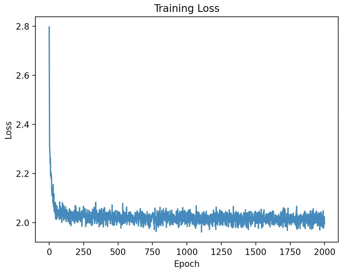
  • 训练 Loss 变化趋势

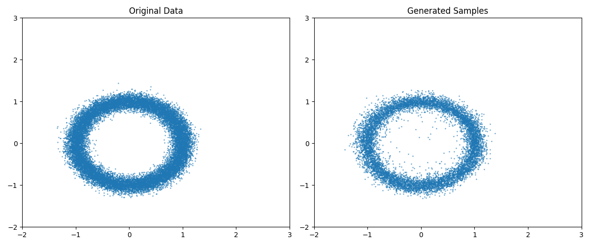
  • 真实值(左)对比采样值(右):

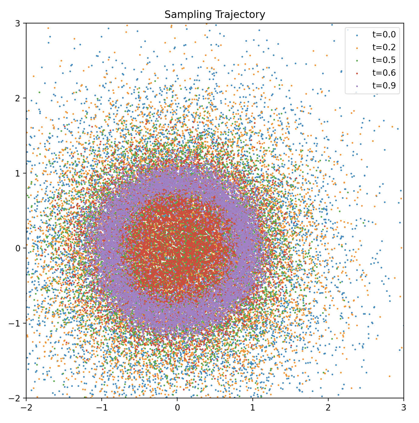
  • 采样过程展示(从图中可看出,随着 \(t\) 从 0 到 1 逐渐增大,采样到的点从最开始的随机分布,到后来越来越趋近于目标分布(圆形))
DL——VAE

  • 参考文献:
    • 原始论文:Auto-Encoding Variational Bayes:

VAE整体说明

  • 变分自编码器(Variational Auto-Encoder,VAE)是一种生成式模型,在机器学习和深度学习领域有广泛应用

VAE的问题设定

  • 给定观测数据 \( \mathbf{x} \),假设其由隐变量 \( \mathbf{z} \) 生成,联合分布为 \( p_\theta(\mathbf{x}, \mathbf{z}) = p_\theta(\mathbf{x}|\mathbf{z}) p(\mathbf{z}) \),其中:
    • \( p(\mathbf{z}) \) 是隐变量的先验分布(通常为标准正态 \( \mathcal{N}(0, I) \))
    • \( p_\theta(\mathbf{x}|\mathbf{z}) \) 是生成模型(解码器),参数为 \( \theta \)
  • 目标:最大化观测数据的边际似然 \( p_\theta(\mathbf{x}) = \int p_\theta(\mathbf{x}|\mathbf{z}) p(\mathbf{z}) d\mathbf{z} \),但积分难计算

一些设想(基本推导思路,可以跳过)

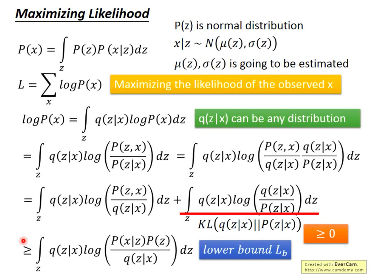
  • 为了最大化概率 \(\sum_{x}\log P(x)\),可先进行如下推导:
    $$
    \begin{align}
    L&=\sum_{x}\log P(x)\\
    &=\int_{z}q(z|x)\cdot\log P(x)dz\\
    &=\int_{z}q(z|x)\cdot\log\left(\frac{p(z,x)}{p(z|x)}\right)dz\\
    &=\int_{z}q(z|x)\cdot\log\left(\frac{p(z,x)}{q(z|x)}\cdot\frac{q(z|x)}{p(z|x)}\right)dz\\
    &=\int_{z}q(z|x)\cdot\log\left(\frac{p(z,x)}{q(z|x)}\right)dz+\underbrace{\int_{z}q(z|x)\cdot\log\left(\frac{q(z|x)}{p(z|x)}\right)dz}_{KL(q(z|x)||p(z|x))\geq0}\\
    &\geq\int_{z}q(z|x)\cdot\log\left(\frac{p(z,x)}{q(z|x)}\right)dz\\
    &=\int_{z}q(z|x)\cdot\log\left(\frac{p(x|z)\cdot p(z)}{q(z|x)}\right)dz\\
    &=\underbrace{\int_{z}q(z|x)\cdot\log(p(x|z))dz}_{Entropy}+\underbrace{\int_{z}q(z|x)\cdot\log\left(\frac{p(z)}{q(z|x)}\right)dz}_{-KL(q(z|x)||p(z))}
    \end{align}
    $$
    • 上述推导说明,最大化似然函数 \(L = \sum_{x}\log P(x)\) 可变成最大化:
      $$L’ = \int_{z}q(z|x)\cdot\log(p(x|z))dz + \int_{z}q(z|x)\cdot\log\left(\frac{p(z)}{q(z|x)}\right)dz$$
      • 实际上,后续会提到 \(L’\) 就是 \(L\) 的变分下界

VAE的推导

  • 引入变分分布 \( q_\phi(\mathbf{z}|\mathbf{x}) \)(编码器),近似真实后验 \( p_\theta(\mathbf{z}|\mathbf{x}) \),参数为 \( \phi \)。通过最小化 \( q_\phi(\mathbf{z}|\mathbf{x}) \) 与 \( p_\theta(\mathbf{z}|\mathbf{x}) \) 的KL散度:
    $$
    \min_{\phi} D_{\text{KL} }\left(q_\phi(\mathbf{z}|\mathbf{x}) | p_\theta(\mathbf{z}|\mathbf{x})\right)
    $$
  • 展开KL散度:
    $$
    D_{\text{KL} }\left(q_\phi(\mathbf{z}|\mathbf{x}) | p_\theta(\mathbf{z}|\mathbf{x})\right) = \mathbb{E}_{q_\phi(\mathbf{z}|\mathbf{x})} \left[ \log q_\phi(\mathbf{z}|\mathbf{x}) - \log p_\theta(\mathbf{z}|\mathbf{x}) \right]
    $$
  • 利用贝叶斯公式 \( p_\theta(\mathbf{z}|\mathbf{x}) = \frac{p_\theta(\mathbf{x}|\mathbf{z}) p(\mathbf{z})}{p_\theta(\mathbf{x})} \),代入得:
    $$
    D_{\text{KL} }\left(q_\phi(\mathbf{z}|\mathbf{x}) | p_\theta(\mathbf{z}|\mathbf{x})\right) = \mathbb{E}_{q_\phi(\mathbf{z}|\mathbf{x})} \left[ \log q_\phi(\mathbf{z}|\mathbf{x}) - \log p_\theta(\mathbf{x}|\mathbf{z}) - \log p(\mathbf{z}) \right] + \log p_\theta(\mathbf{x})
    $$
  • 整理后得到:
    $$
    \log p_\theta(\mathbf{x}) - D_{\text{KL} }\left(q_\phi(\mathbf{z}|\mathbf{x}) | p_\theta(\mathbf{z}|\mathbf{x})\right) = \mathbb{E}_{q_\phi(\mathbf{z}|\mathbf{x})} \left[ \log p_\theta(\mathbf{x}|\mathbf{z}) \right] - D_{\text{KL} }\left(q_\phi(\mathbf{z}|\mathbf{x}) | p(\mathbf{z})\right)
    $$

证据下界(ELBO)

  • 证据下界(Evidence Lower Bound, ELBO),也称为变分下界(Variational Lower Bound, VLB)
  • 由于 \( D_{\text{KL} } \geq 0 \),有:
    $$
    \log p_\theta(\mathbf{x}) \geq \underbrace{\mathbb{E}_{q_\phi} \left[ \log p_\theta(\mathbf{x}|\mathbf{z}) \right] - D_{\text{KL} }\left(q_\phi(\mathbf{z}|\mathbf{x}) | p(\mathbf{z})\right)}_{\text{ELBO}(\theta, \phi)}
    $$
  • 目标转为最大化ELBO:
    $$
    \mathcal{L}(\theta, \phi; \mathbf{x}) = \mathbb{E}_{q_\phi(\mathbf{z}|\mathbf{x})} \left[ \log p_\theta(\mathbf{x}|\mathbf{z}) \right] - D_{\text{KL} }\left(q_\phi(\mathbf{z}|\mathbf{x}) | p(\mathbf{z})\right)
    $$
    • 此时,最大化ELBO \(\mathcal{L}(\theta, \phi; \mathbf{x})\) 就可以实现最大化原始对数似然函数目标 \(\log p_\theta(\mathbf{x})\)
    • ELBO的更多等价形式见附录

损失函数分解(ELBO包含两项)

  • 1. 重构项(Reconstruction Term)最大化 :
    $$
    \mathbb{E}_{q_\phi(\mathbf{z}|\mathbf{x})} \left[ \log p_\theta(\mathbf{x}|\mathbf{z}) \right]
    $$

    • 作用:鼓励解码器重建输入数据,通常用均方误差(MSE)或交叉熵实现
    • 理解:最大化\(\mathbb{E}_{q_\phi(\mathbf{z}|\mathbf{x})} \left[ \log p_\theta(\mathbf{x}|\mathbf{z}) \right]\)等价于上面的公式等价于:
      • 从原始数据集 \(\mathcal{D}\) 任意采样一个数据 \(\mathbf{x}_0\);
      • 经过编码器 \(q_\phi(\mathbf{z}|\mathbf{x})\) 将 \(\mathbf{x}_0\) 编码成 \(\mathbf{z}\),其中 \(\mathbf{z} \sim q_\phi(\mathbf{z}|\mathbf{x}_0)\);
      • 再经过解码器 \(p_\theta(\mathbf{x}|\mathbf{z})\) 将编码器的输出 \(\mathbf{z}\) 解码成 \(\mathbf{x}_i\)
      • 最大化 \(\log p_\theta(\mathbf{x}|\mathbf{z})\),等价于最小化 \(\mathbf{x}_i\) 和 \(\mathbf{x}_0\) 的距离(常用交叉熵损失或者MSE)
  • 2. 正则项(KL Divergence Term)最小化 :
    $$
    D_{\text{KL} }\left(q_\phi(\mathbf{z}|\mathbf{x}) | p(\mathbf{z})\right)
    $$

    • 作用:约束编码器输出接近先验分布 \( p(\mathbf{z}) \),避免过拟合
    • 理解:先验分布 \( p(\mathbf{z}) \)可以设定为任意我们方便采样的值,比如VAE中将其设定为标准正态分布 \(\mathcal{N}(0, I) \)

KL散度的闭式解

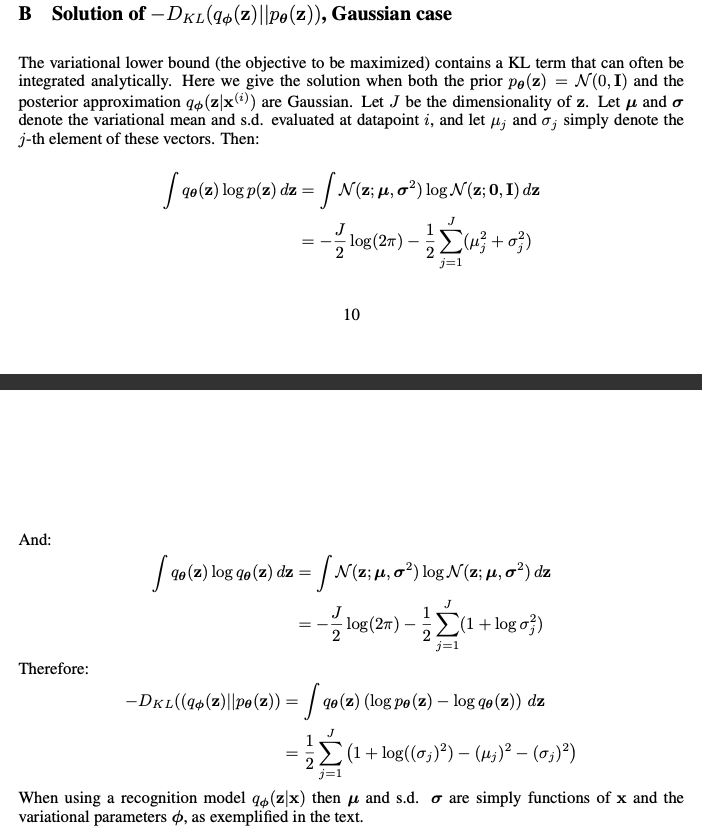
  • 假设 \( p(\mathbf{z}) = \mathcal{N}(0, I) \),且 \( q_\phi(\mathbf{z}|\mathbf{x}) = \mathcal{N}(\mu_\phi(\mathbf{x}), \sigma_\phi^2(\mathbf{x}) I) \),则KL散度有闭式解:
    $$
    D_{\text{KL} }\left(q_\phi(\mathbf{z}|\mathbf{x}) | p(\mathbf{z})\right) = -\frac{1}{2} \sum_{j=1}^J \left(1 + \log \sigma_j^2 - \mu_j^2 - \sigma_j^2\right)
    $$
    • 其中 \( J \) 是隐变量维度
    • 证明过程见附录

重参数化技巧(Reparameterization Trick)

  • 为可微分地采样 \( \mathbf{z} \sim q_\phi(\mathbf{z}|\mathbf{x}) \),令:
    $$
    \mathbf{z} = \mu_\phi(\mathbf{x}) + \sigma_\phi(\mathbf{x}) \odot \epsilon, \quad \epsilon \sim \mathcal{N}(0, I)
    $$
    • 使得梯度可回传

最终损失函数(负 ELBO)

  • 总损失函数 :
    $$
    \mathcal{L}_{\text{VAE} }(\theta, \phi; \mathbf{x}) = \underbrace{\mathbb{E}_{q_\phi(\mathbf{z}|\mathbf{x})} \left[ -\log p_\theta(\mathbf{x}|\mathbf{z}) \right]}_{\text{Reconstruction Loss} } + \underbrace{D_{\text{KL} }\left(q_\phi(\mathbf{z}|\mathbf{x}) | p(\mathbf{z})\right)}_{\text{KL Divergence} }
    $$
    • 重构损失采用 MSE 或交叉熵损失函数:
      $$
      \text{Reconstruction Loss} = |\mathbf{x} - \text{Decoder}(\text{Encoder}(\mathbf{x}))|_2^2
      $$
    • KL 散度闭式解(假设 \( q_\phi(\mathbf{z}|\mathbf{x}) = \mathcal{N}(\mu, \sigma^2) \)):
      $$
      D_{\text{KL} }\left(q_\phi(\mathbf{z}|\mathbf{x}) | p(\mathbf{z})\right) = - \frac{1}{2} \sum_{j=1}^J \left( 1 + \log \sigma_j^2 - \mu_j^2 - \sigma_j^2 \right)
      $$
      • 其中 \( J \) 是隐变量维度
  • 最终,VAE的最终版MSE版损失函数为:
    $$
    \begin{align}
    \mathcal{L}_{\text{VAE} }(\theta, \phi; \mathbf{x}) &= \text{Reconstruction Loss} + D_{\text{KL} }\left(q_\phi(\mathbf{z}|\mathbf{x}) | p(\mathbf{z})\right) \\
    &= |\mathbf{x} - \text{Decoder}(\text{Encoder}(\mathbf{x}))|_2^2 - \frac{1}{2} \sum_{j=1}^J \left( 1 + \log \sigma_j^2 - \mu_j^2 - \sigma_j^2 \right)
    \end{align}
    $$
  • 总体来说:VAE通过最大化ELBO,同时优化生成模型 \( p_\theta(\mathbf{x}|\mathbf{z}) \) 和推断模型 \( q_\phi(\mathbf{z}|\mathbf{x}) \),平衡了数据重建与隐变量正则化

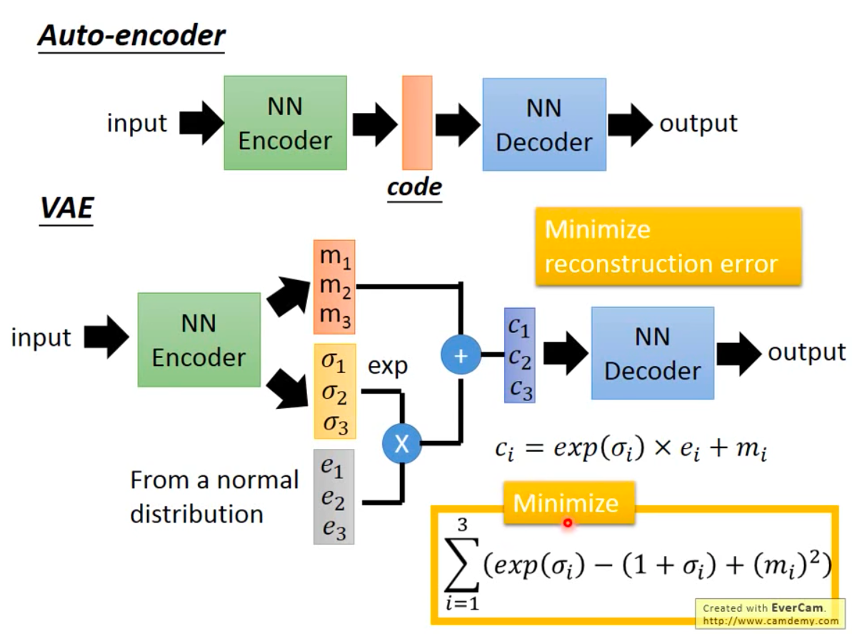
VAE网络结构

  • 下面的网络输出对数方差(能保证方差非负),但是仍然使用 \(\sigma\),容易让人误解,此时使用 \(e^\sigma\) 表示方差,此时有 \(\sigma\) 就是对数方差(原\(\log \sigma^2\))

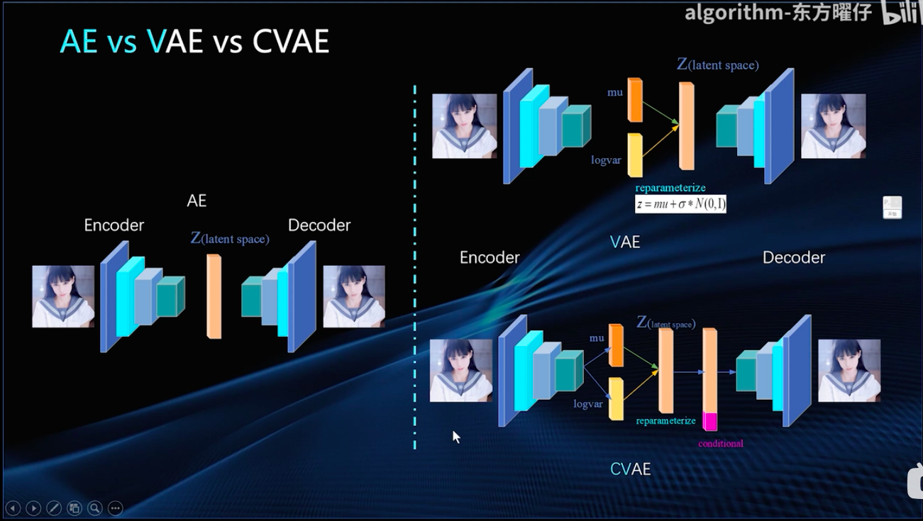
AE-VAE-CVAE

  • AE-VAE-CVAE结构差异:

VAE的简单代码实现

  • 代码实现如下:
    1
    2
    3
    4
    5
    6
    7
    8
    9
    10
    11
    12
    13
    14
    15
    16
    17
    18
    19
    20
    21
    22
    23
    24
    25
    26
    27
    28
    29
    30
    31
    32
    33
    34
    35
    36
    37
    38
    39
    40
    41
    42
    43
    44
    45
    46
    47
    48
    49
    50
    51
    52
    53
    54
    55
    56
    57
    58
    59
    60
    61
    62
    63
    64
    65
    66
    67
    68
    69
    70
    71
    72
    73
    74
    75
    76
    77
    78
    79
    80
    81
    82
    83
    84
    85
    86
    87
    88
    89
    90
    91
    92
    93
    94
    95
    import torch
    import torch.nn as nn
    import torch.optim as optim
    from torchvision import datasets, transforms
    import torchvision.utils as vutils
    import matplotlib.pyplot as plt

    # 定义 VAE 模型
    class VAE(nn.Module):
    def __init__(self, input_size, hidden_size=400, latent_size=20):
    super(VAE, self).__init__()

    # 编码器
    self.fc1 = nn.Linear(input_size, hidden_size)
    self.fc_mu = nn.Linear(hidden_size, latent_size)
    self.fc_logvar = nn.Linear(hidden_size, latent_size)

    # 解码器
    self.fc2 = nn.Linear(latent_size, hidden_size)
    self.fc3 = nn.Linear(hidden_size, input_size)

    def encode(self, x):
    h = torch.relu(self.fc1(x))
    return self.fc_mu(h), self.fc_logvar(h)

    def reparameterize(self, mu, logvar):
    std = torch.exp(0.5 * logvar)
    eps = torch.randn_like(std)
    return mu + eps * std

    def decode(self, z):
    h = torch.relu(self.fc2(z))
    return torch.sigmoid(self.fc3(h))

    def forward(self, x):
    mu, logvar = self.encode(x.view(-1, 784))
    z = self.reparameterize(mu, logvar)
    return self.decode(z), mu, logvar


    # 定义损失函数
    def loss_function(recon_x, x, mu, logvar):
    BCE = nn.functional.binary_cross_entropy(recon_x, x.view(-1, 784), reduction='sum')
    KLD = -0.5 * torch.sum(1 + logvar - mu.pow(2) - logvar.exp())
    return BCE + KLD


    # 训练函数
    def train(model, train_loader, optimizer, epoch):
    model.train()
    train_loss = 0
    for batch_idx, (data, _) in enumerate(train_loader):
    data = data.to(device)
    optimizer.zero_grad()
    recon_batch, mu, logvar = model(data)
    loss = loss_function(recon_batch, data, mu, logvar)
    loss.backward()
    train_loss += loss.item()
    optimizer.step()
    print(f'====> Epoch: {epoch} Average loss: {train_loss / len(train_loader.dataset):.4f}')


    # 生成图片函数
    def generate_image(model, device):
    model.eval()
    with torch.no_grad():
    z = torch.randn(1, 20).to(device)
    sample = model.decode(z).cpu()
    sample = sample.view(1, 1, 28, 28)
    vutils.save_image(sample, 'generated_image.png')
    plt.imshow(sample.squeeze().numpy(), cmap='gray')
    plt.show()


    # 数据加载
    transform = transforms.Compose([
    transforms.ToTensor()
    ])
    train_dataset = datasets.MNIST(root='./data', train=True, transform=transform, download=True)
    train_loader = torch.utils.data.DataLoader(train_dataset, batch_size=128, shuffle=True)

    # 设备配置
    device = torch.device("cuda" if torch.cuda.is_available() else "cpu")

    # 初始化模型、优化器
    model = VAE(input_size=784).to(device)
    optimizer = optim.Adam(model.parameters(), lr=1e-3)

    # 训练模型
    num_epochs = 10
    for epoch in range(1, num_epochs + 1):
    train(model, train_loader, optimizer, epoch)

    # 生成图片
    generate_image(model, device)

附录:VAE李宏毅公式推导

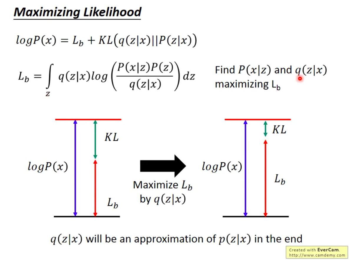
  • 目标是让似然函数最大化,也就是最大化 \(\sum_x \log P(x)\),推导可得相当于最大化变分下界(Evidence Lower Bound, \(ELBO(q)\))
  • 为什么要通过求解 \(q\) 来实现似然函数最大化/ELBO最大化呢?因为优化 \(q\) 时,与 \(P(x)\) 无关,相当于最小化KL散度
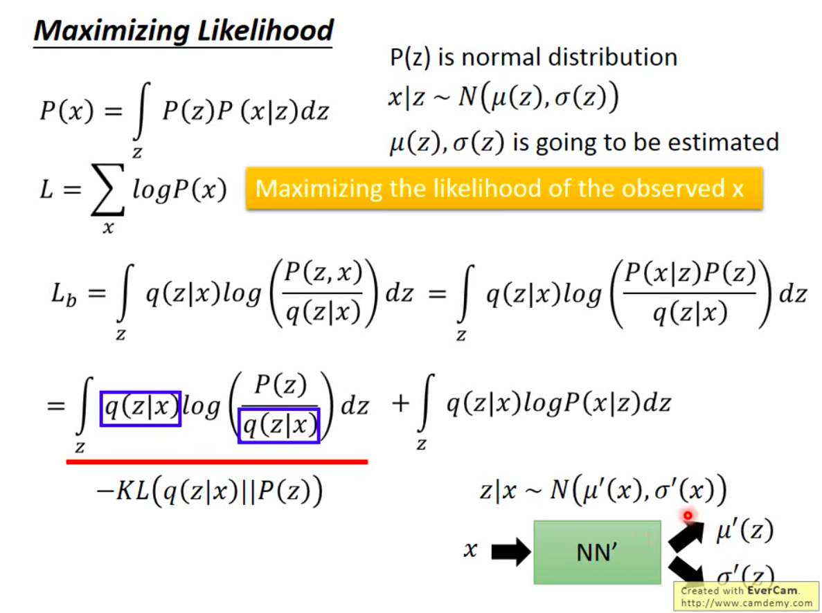
  • 进一步拆解变分下界
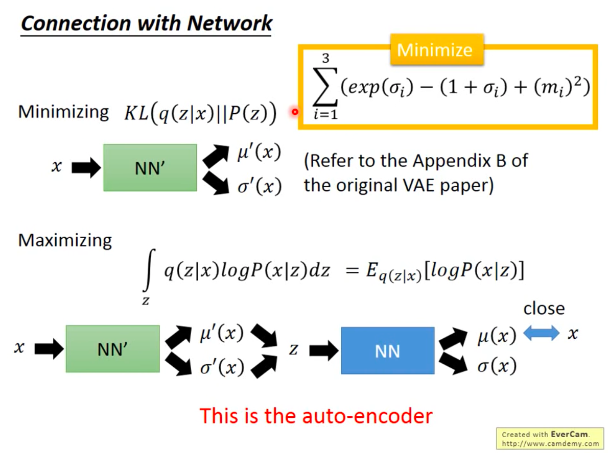
  • 变分下界的两个部分分别可用在网络中建模,两个损失函数同时优化就是VAE * 期望部分:通过带采样的Auto-Encoder实现,损失函数为Auto-Encoder的损失函数
附录:KL散度闭市解的推导

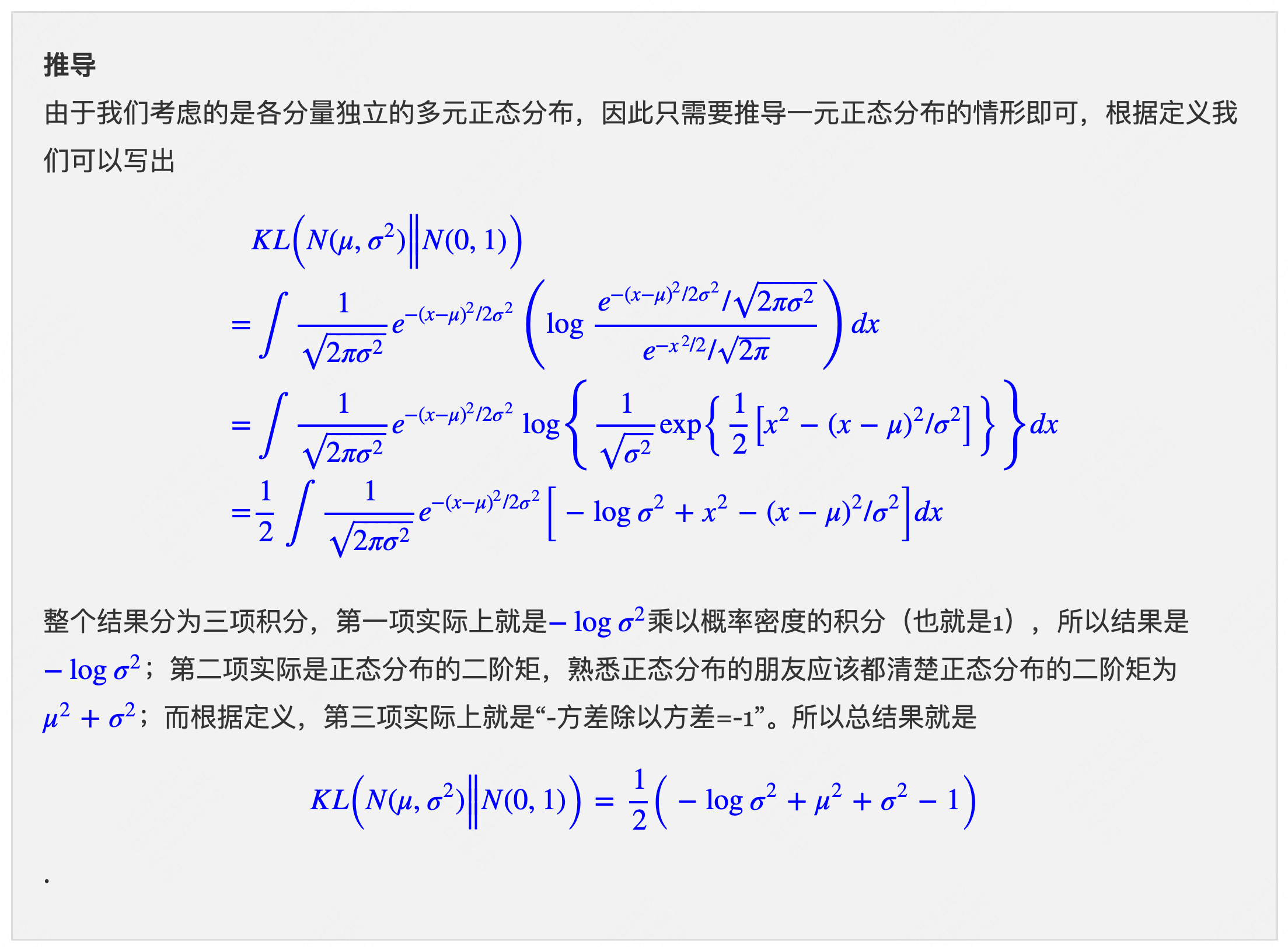
  • 假设 \(p(z)\) 是均值为0方差为1的标准正太分布 \(N(0,I)\),所以这里KL散度本质是要尽量保证分布 \(q(z|x)\) 尽可能接近标准正太分布,使用一个关于均值和方差的损失函数可以实现
  • KL散度部分的闭市解推导,来自 苏神的科学空间:
  • 原始论文推导可见:Auto-Encoding Variational Bayes:

附录:ELBO的各种等价形式

  • 一些等价形式:一些推导中会涉及到ELBO的不同形式:
    $$
    \begin{align}
    \mathcal{L}(\theta, \phi; \mathbf{x}) &= \mathbb{E}_{q_\phi(\mathbf{z}|\mathbf{x})} \left[ \log p_\theta(\mathbf{x}|\mathbf{z}) \right] - D_{\text{KL} }\left(q_\phi(\mathbf{z}|\mathbf{x}) | p(\mathbf{z})\right) \\
    &= \mathbb{E}_{q_\phi(\mathbf{z}|\mathbf{x})} \left[ \log p_\theta(\mathbf{x}|\mathbf{z}) \right] - \mathbb{E}_{q_\phi(\mathbf{z}|\mathbf{x})}\left[\frac{\log q_\phi(\mathbf{z}|\mathbf{x})}{\log p(\mathbf{z})}\right] \\
    &= \mathbb{E}_{q_\phi(\mathbf{z}|\mathbf{x})} \left[ \log p_\theta(\mathbf{x}|\mathbf{z}) \frac{\log p(\mathbf{z})}{\log q_\phi(\mathbf{z}|\mathbf{x})}\right] \\
    &= \mathbb{E}_{q_\phi(\mathbf{z}|\mathbf{x})} \left[ \log p_\theta(\mathbf{x}|\mathbf{z}) \frac{\log p(\mathbf{z})}{\log q_\phi(\mathbf{z}|\mathbf{x})}\right] \\
    &= \mathbb{E}_{q_\phi(\mathbf{z}|\mathbf{x})} \left[ \frac{\log p_\theta(\mathbf{x},\mathbf{z})}{\log q_\phi(\mathbf{z}|\mathbf{x})}\right] \\
    \end{align}
    $$
1…248249250…352
San Ye

San Ye

Stay Hungry. Stay Foolish.

704 posts
53 tags
© 2026 San Ye
Powered by Hexo
|
Theme — NexT.Gemini v5.1.4