Hexo

凡事预则立,不预则废


  • Home

  • Tags

  • Archives

  • Navigation

  • Search

RL——Decision-Transformer

Decision-Transformer,简称DT,使用序列预估的思想去实现决策问题

  • 参考链接:
    • 原始论文:Decision Transformer: Reinforcement Learning via Sequence Modeling, UC Berkeley, NuerIPS 2021
    • 源码:github.com/kzl/decision-transformer

HER 技术

  • 在 Decision Transformer 之前,HER(Hindsight Experience Replay)方法已经有这种事后的思想,HER 过将想要达到的目标状态添加到策略网络的输入端,实现在给定目标的情况下,进行决策

Decision Transformer

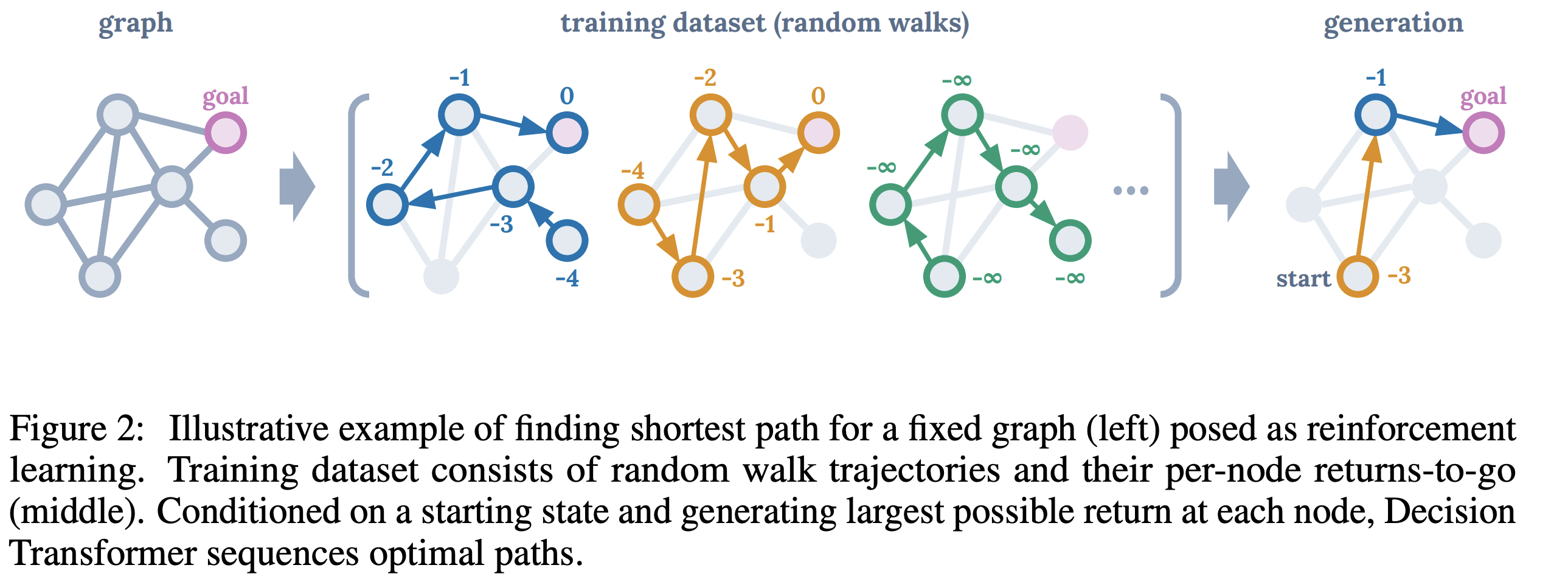
returns-to-go轨迹变换

  • 原始的轨迹: \( \tau = (s_1,a_1,r_1,s_2,a_2,r_2,\cdots,s_T,a_T,r_T) \)
  • returns-to-go对应的轨迹: \( \tau = (\hat{R}_1,s_1,a_1,\hat{R}_2,s_2,a_2,\cdots,\hat{R}_T,s_T,a_T) \)
    • \(\hat{R}_t = \sum_{t’=t}^T r_{t’}\) 被称为return-to-go(与state、action等一样的粒度),表示复数或者泛指时,也是用returns-to-go
    • 注意, \(\hat{R}_t\) 没有使用discount ratio,是无折扣的奖励,方便后续实现中减去已获得的奖励实现目标值变换

建模方式

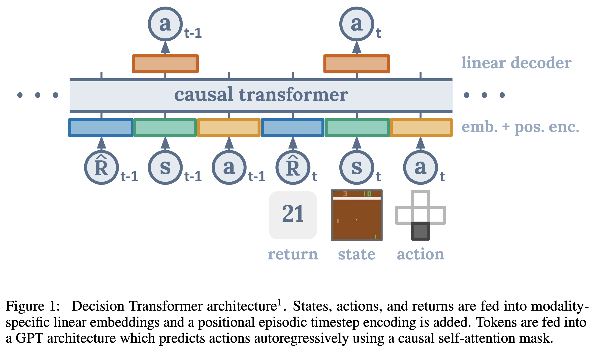
  • 整体架构
  • demo

伪代码

  • 在原始 Transformer 的基础上,DT 算法的实现非常简单,DT 算法的整体伪代码如下(连续版本):

    1
    2
    3
    4
    5
    6
    7
    8
    9
    10
    11
    12
    13
    14
    15
    16
    17
    18
    19
    20
    21
    22
    23
    24
    25
    26
    27
    28
    29
    30
    31
    32
    33
    34
    35
    36
    37
    38
    39
    40
    41
    42
    43
    # R, s, a, t: returns -to -go, states, actions, or timesteps
    # K: context length (length of each input to DecisionTransformer)
    # transformer: transformer with causal masking (GPT)
    # embed_s, embed_a, embed_R: linear embedding layers
    # embed_t: learned episode positional embedding
    # pred_a: linear action prediction layer

    # main model
    def DecisionTransformer(R, s, a, t):
    # compute embeddings for tokens
    pos_embedding = embed_t(t) # per -timestep (note: not per -token)
    a_embedding = embed_a(a) + pos_embedding
    s_embedding = embed_s(s) + pos_embedding
    R_embedding = embed_R(R) + pos_embedding
    # interleave tokens as (R_1, s_1, a_1, ..., R_K, s_K)
    input_embeds = stack(R_embedding, s_embedding, a_embedding)
    # use transformer to get hidden states
    hidden_states = transformer(input_embeds=input_embeds)
    # select hidden states for action prediction tokens
    a_hidden = unstack(hidden_states).actions
    # predict action
    return pred_a(a_hidden)


    # training loop
    for (R, s, a, t) in dataloader: # dims: (batch_size, K, dim)
    a_preds = DecisionTransformer(R, s, a, t)
    loss = mean((a_preds - a) ** 2) # L2 loss for continuous actions
    optimizer.zero_grad()
    loss.backward()
    optimizer.step()

    # evaluation loop
    target_return = 1 # for instance, expert -level return
    R, s, a, t, done = [target_return], [env.reset()], [], [1], False
    while not done: # autoregressive generation/sampling
    # sample next action
    action = DecisionTransformer(R, s, a, t)[-1] # for cts actions
    new_s, r, done, _ = env.step(action)
    # append new tokens to sequence
    R = R + [R[-1] - r] # decrement returns -to -go with reward
    s, a, t = s + [new_s], a + [action], t + [len(R)]
    R, s, a, t = R[-K:], s[-K:], a[-K:], t[-K:] # only keep context length of K
  • 伪代码讲解:

    • token:包含三种模态的token,分别为return-to-go、state和action
    • 位置编码:虽然是三个token,但是同一个时间片的return-to-go、state和action,对应的位置编码相同
    • 模型的输入:过去 \(K-1\) 个时间片的(return-to-go,state,action)完整信息和当前时间片的(return-to-go,state),共 \((K-1)*3+2\) 个tokens
    • 输出:仅在输入是state token对应的位置上,输出action token为决策目标
    • 损失函数:伪代码中使用的是MSE损失函数(对应连续动作场景),实际上对于离散动作场景, 可以使用交叉熵损失函数(策略网络输出Softmax后的多个头)
    • 训练时:
      • 每个样本仅保留最近的 \(K\) 个步骤,模型输入是 \(K*\) 个样本
      • 时间步 \(t\) 是一直累计的,与 \(K\) 无关
    • 推断时的自回归:
      • 初始化时先指定初始状态 \(s_0\) 和最终目标target_return \(R_0\)
      • 通过DT模型决策得到动作 \(a_t\)
      • 与环境交互执行动作 \(a_t\) 并得到reward \(r_{t}\),并跳转到状态 \(s_{t+1}\)
      • 通过reward \(r_t\) 计算下个时间步的return-to-go \(R_{t+1} = R_t - r_t\)
      • 将 \((a_t, s_{t+1}, R_{t+1})\) 分别加入到各自token列表中
      • 截断到 \(K\) 个时间步,注意动作是保留 \(K-1\) 个,不足 \(K\) 个时间步时,会自动paddding(直接调用Transformer)即可,此时也需要保证模型输入action比return-to-go和state少一个

预测时如何指定Reward目标?

  • 可以使用离线采样样本中Reward最大值作为目标,论文原始表述如下

  • 个人理解:这个目标不一定要是最优目标,也不需要与离线目标完全相等,但是比较难设置:

    • 如果太小,但是生成的不一定是最优的路径
    • 如果太大,理论上,可以生成最优解,但是因为模型没有见过该目标值(模型做不到,因为训练时也收集不到这样的样本),可能会发生意想不到情况

实验结果

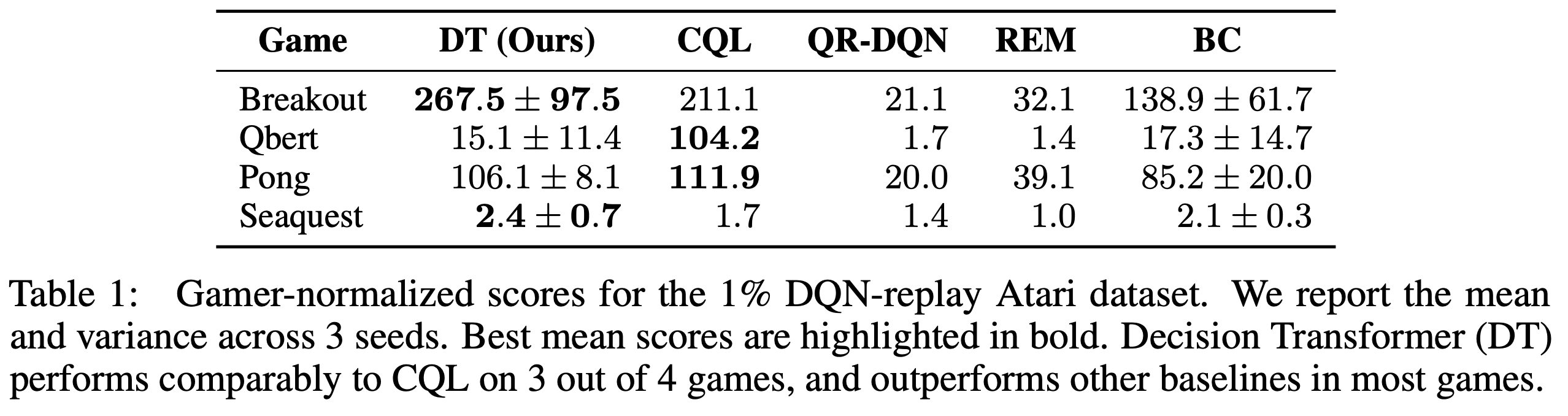
  • Atari上收集的实验数据集训练的实验结果见如下图:

    • 在部分场景上,CQL效果更好
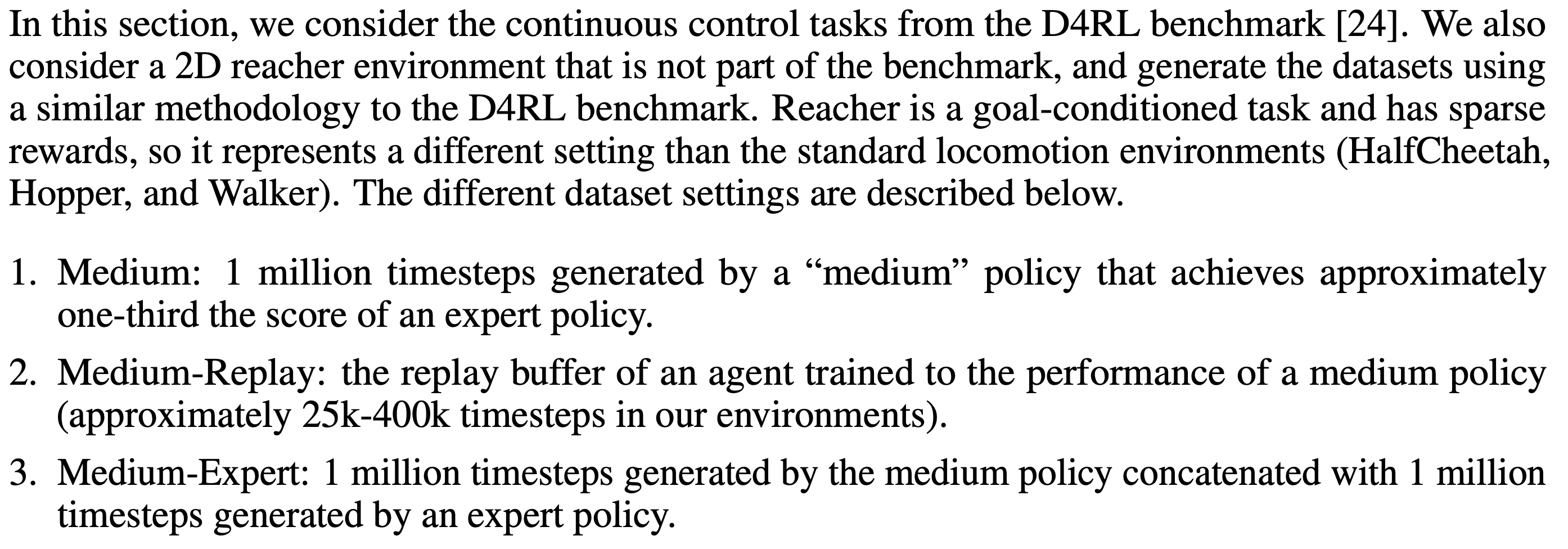
  • D4RL以及OpenAI-Gym上收集的数据集上的实验结果如下图(注意,补充了一些):
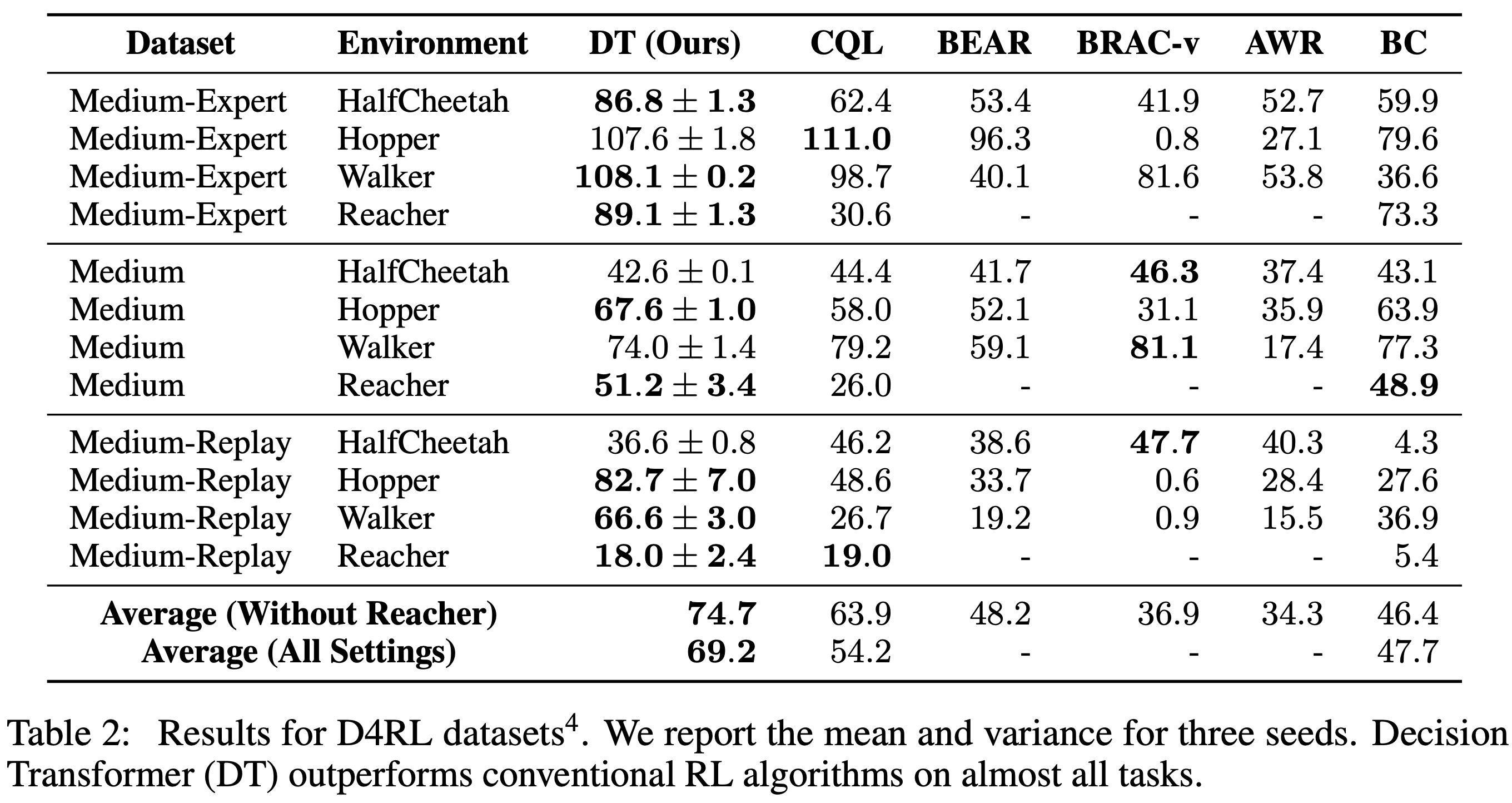
    • 补充了一些D4RL中没有的数据集(Medium是指直接用Medium Agent与环境交互生成的样本;Medium-Replay是指训练一个Medium Agent时收集的Replay Buffer;Medium-Expert是Medium Agent和Expert Agent两种策略收集到的数据集的混合)
RL——Decision-Diffuser

Decision-Diffuser

  • 参考链接:
    • 原始论文:Is Conditional Generative Modeling all you need for Decision-Making?, MIT, ICLR 2023
    • 源码:github.com/anuragajay/decision-diffuser
    • 官方博客:anuragajay.github.io/decision-diffuser
    • 参考链接:Diffusion Model + RL 系列技术科普博客(2):Decision Diffuser - DILab决策实验室的文章 - 知乎
    • Classifier-Free Diffusion Guidance, Google Research, Brain team, 2022,Classifier-Free Guidance方法

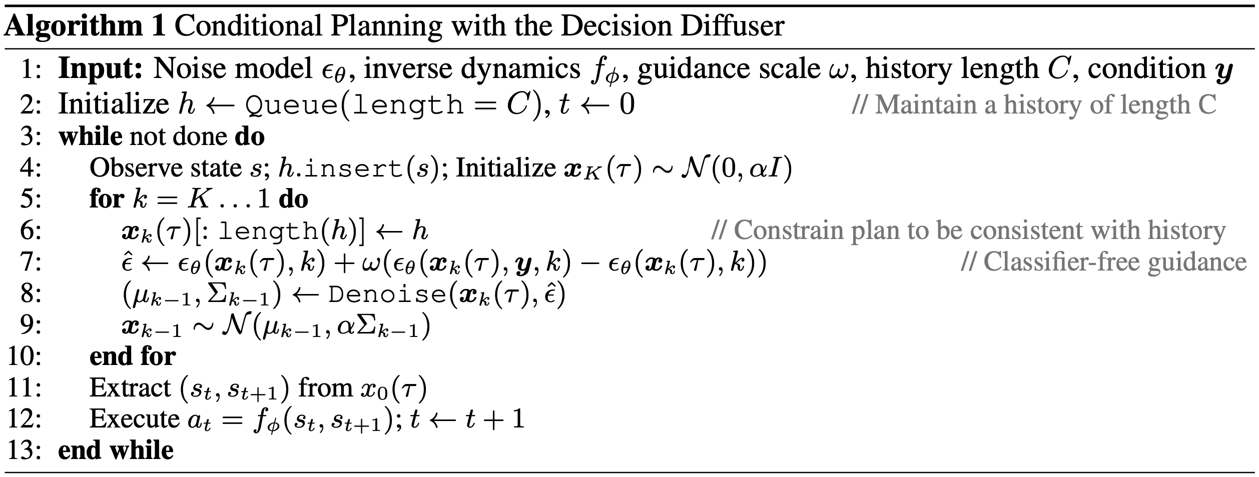
核心贡献点总结(对比 Diffuser)

  • 序列组织方式 :
    • Diffuser的序列包含了状态和动作
    • Decision Diffuser的序列仅包含状态,不包含动作 ,这样做的原因是强化学习的状态往往是连续且平滑的,动作则往往是离散或结构化的,此外一些动作可能变化很高,很不平滑,Diffusion模型难以建模
  • Guidance 方法 :
    • Diffuser使用Classifier Guidance的方法
    • Decision Diffuser采用Classifier-free Guidance的方法
  • 决策过程中的历史轨迹窗口 :
    • Diffuser使用历史长度为1的滑动窗口 ,在每个Diffusion采样时间步,每次仅保留单个历史状态 \(s_0\)
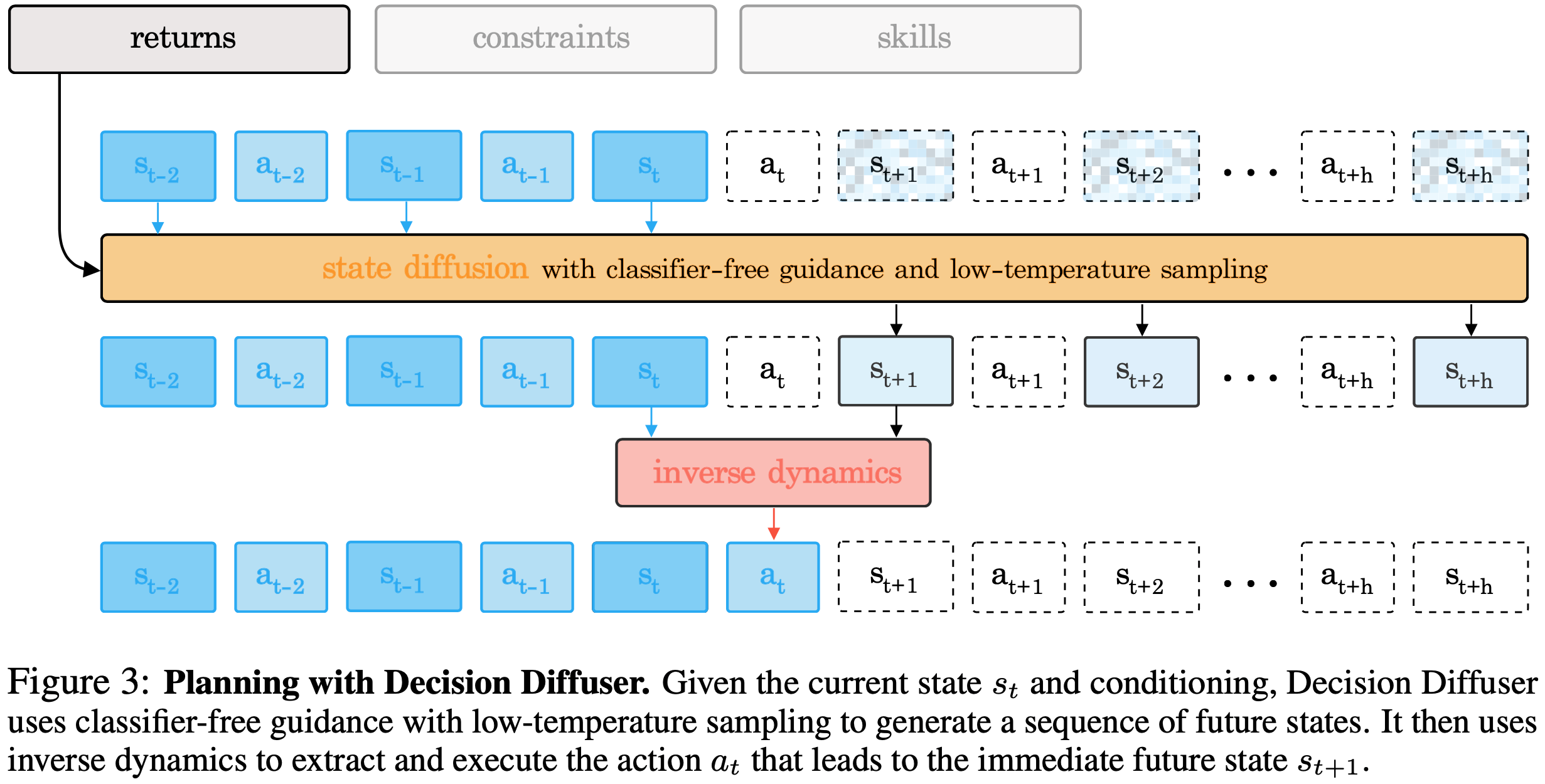
    • Decision Diffuser使用历史长度为C的滑动窗口 ,在每个Diffusion采样时间步,Decision Diffuser将最近C个历史状态(实验中设置为C=20,planning horizon则根据不同的任务设置不同的值),直接赋值给当前的轨迹的前半部分,类似图片补全功能,保证生成后续的轨迹与当前轨迹一致
  • 决策方式 :
    • Diffuser直接按照轨迹生成的动作决策
    • Decision Diffuser在轨迹中不直接生成动作,而是在生成轨迹中提取出 \(s_t,s_{t+1}\) 后,使用一个专门训练的策略网络 \(a_t:= f_\phi(s_t,s_{t+1})\) 来决策动作,网络也称为逆向动力学模型(Acting with Inverse-Dynamics),实际上,在其他文章,还可以是使用更多的状态来生成动作,比如AIGB中使用 \(a_t:= f_\phi(s_{t-L:t},s_{t+1})\)
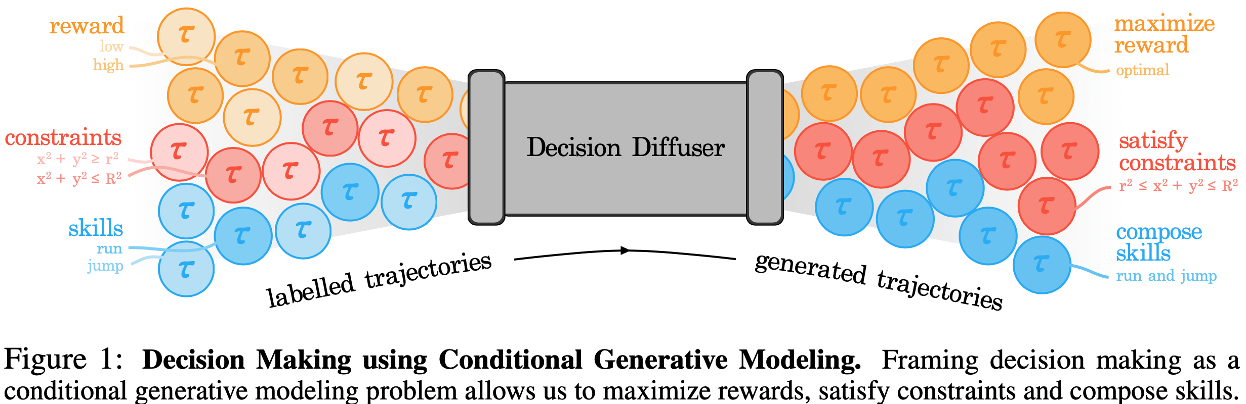
  • 支持不同条件类型:最大化收益、约束满足和组合技能 :
    • 最大化回报(Maximizing Returns) :\(\epsilon_\theta(\boldsymbol{x}_k(\tau), \boldsymbol{y}(\tau), k) := \epsilon_\theta(\boldsymbol{x}_k(\tau), R(\tau), k)\),其中 \(R(\tau) \in [0,1]\) 是经过归一化的奖励函数
    • 约束满足(Satisfying Constraints) :Decision Diffuser条件满足的方式引入约束到网络输入端,具体来说,对于约束 \(\mathcal{C}_i\):\(\epsilon_\theta(\boldsymbol{x}_k(\tau), \boldsymbol{y}(\tau), k) := \epsilon_\theta(\boldsymbol{x}_k(\tau), \mathbb{I}(\tau \in \mathcal{C}_i), k)\),如果包含多个约束,可以使用one-hot向量来训练,满足约束的维度取1,其他维度取0来训练,虽然训练时只见过单约束,但是在采样时可以体现出多约束(one-hot向量变成多维度为1的向量)
    • 组合技能(Skill Composition) :在生成轨迹时,Decision Diffuser可以通过不同Diffusion误差函数相加实现组合技能的采样形式,具体地,对于单一技能定义为:\(\epsilon_\theta(\boldsymbol{x}_k(\tau), \boldsymbol{y}(\tau), k) := \epsilon_\theta(\boldsymbol{x}_k(\tau), \mathbb{I}(\tau \in \mathcal{B}_i), k)\),采样时,多技能组合定义为:
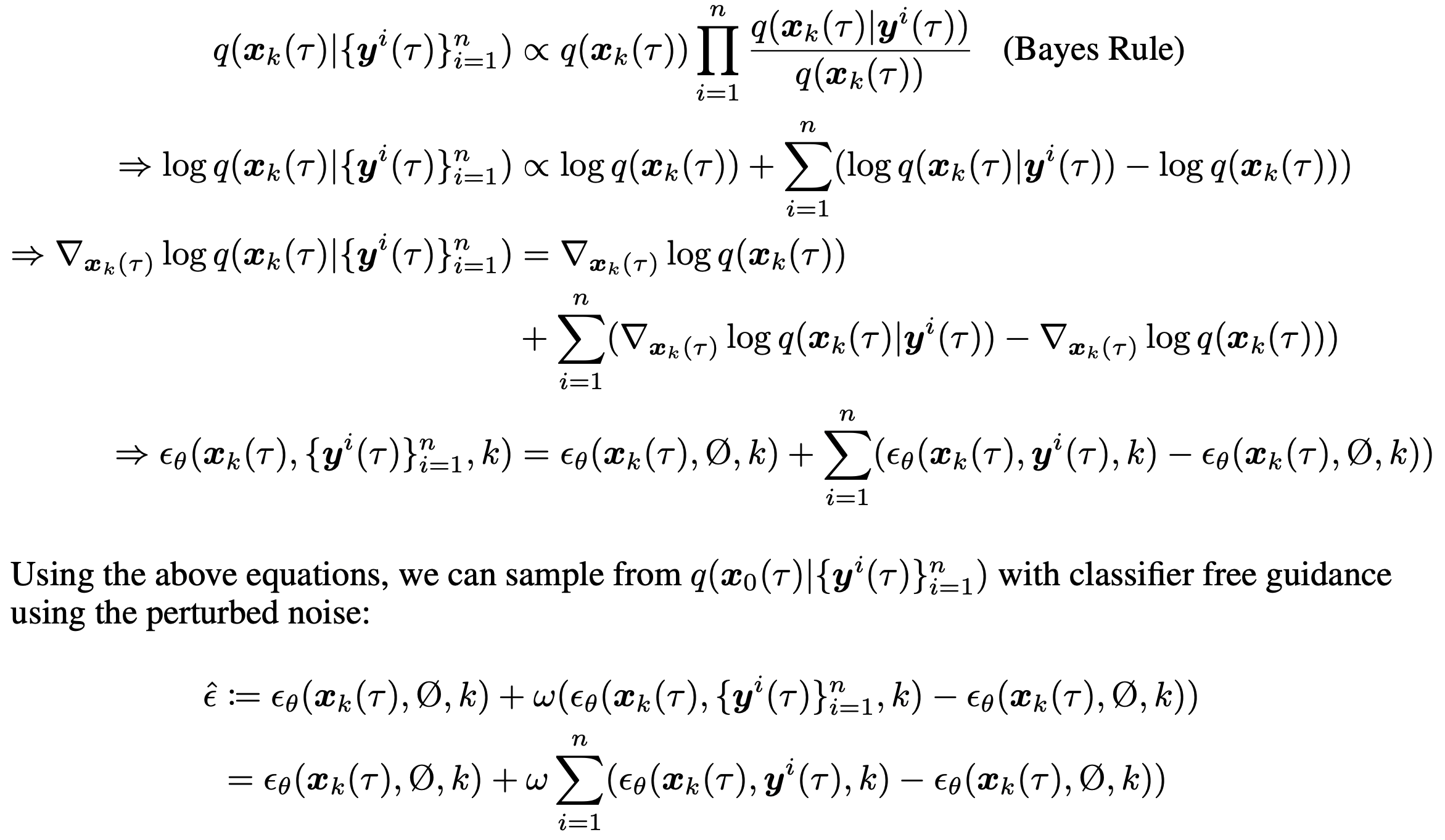
      $$\hat{\epsilon} := \epsilon_\theta(\boldsymbol{x}_k(\tau),\varnothing, k) + \omega \sum_{i=1}^n (\epsilon_\theta(\boldsymbol{x}_k(\tau),\boldsymbol{y}^i(\tau), k) - \epsilon_\theta(\boldsymbol{x}_k(\tau), \varnothing, k))$$
      • 详细推导见附录:多条件组合的证明
    • 其他说明:Decision Diffuser支持约束的“与”运算和“非”运算(做减法),但是不支持或运算(Decision Diffuser 没有为每个条件变量提供显式的密度估计,因此它不能原生支持“或”运算组合)
  • 其他:
    • 低温采样 (Low-temperature Sampling):在常规的扩散模型采样方式中加入一个低温因子 \(\alpha\),即 \(\tau^{i-1} \sim \mathcal{N}(\tau^{i-1}|\mu_\theta(\tau^i, i), \color{red}{\alpha}\Sigma^i)\)

Decision Diffuser 具体实现

建模方式

  • 整体思路概览:
  • 序列组织方式如下:
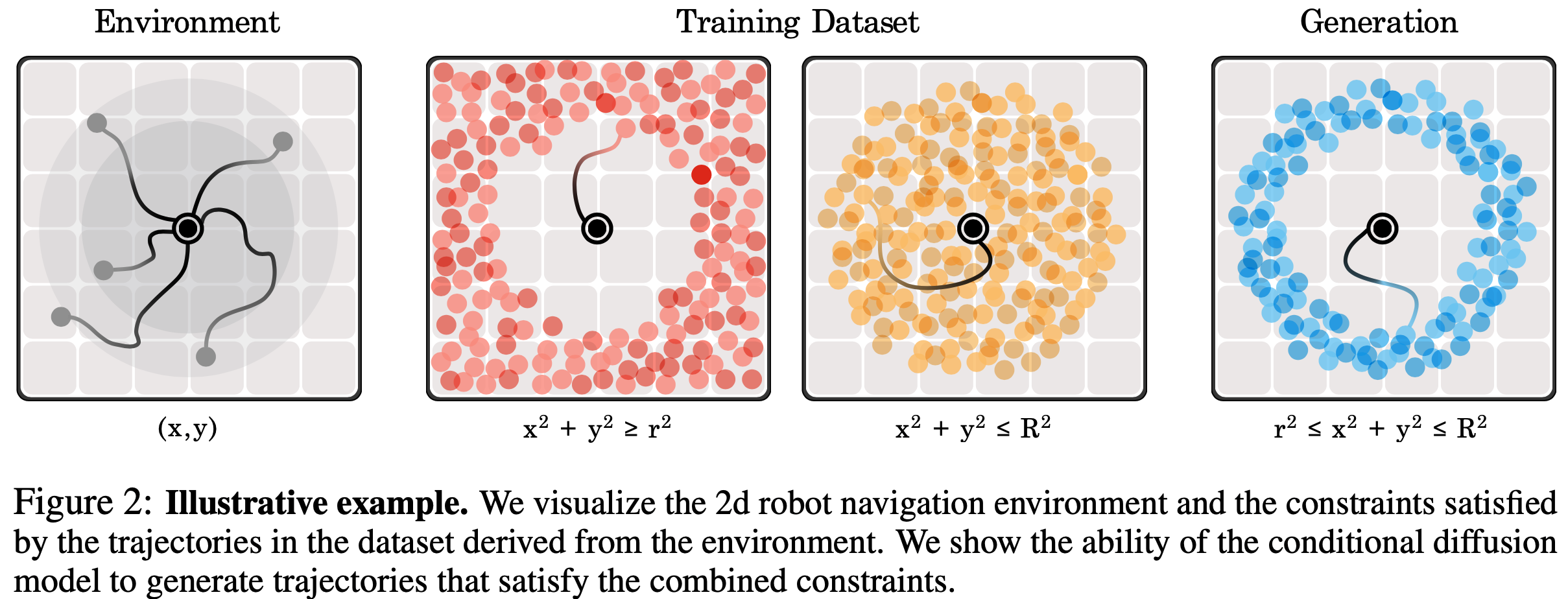
  • 约束同时达成情况示意图:

训练过程

  • 训练过程
    $$ \mathcal{L}(\theta, \phi) := \mathbb{E}_{k, \tau\in\mathcal{D}, \beta\sim\text{Bern}(p)}[||\epsilon - \epsilon_{\theta}(\boldsymbol{x}_{k}(\tau), (1-\beta)\boldsymbol{y}(\tau) + \beta\varnothing, k)||^{2}] + \mathbb{E}_{(s, a, s’) \in \mathcal{D}}[||a-f_{\phi}(s, s’)||^2] $$
  • 两个网络相对独立,实际上写成两个损失函数分别训练也可以的

采样过程

  • Decision Diffuser算法伪代码如下:
  • 其中 \(\hat{\epsilon}\) 的定义与论文Classifier-Free Diffusion Guidance中的方法不同,但事实上通过调整Guidance scale的取值范围,可以得到两者表达式是等价的,详细讨论见附录:关于Guidance scale的讨论

Experiments

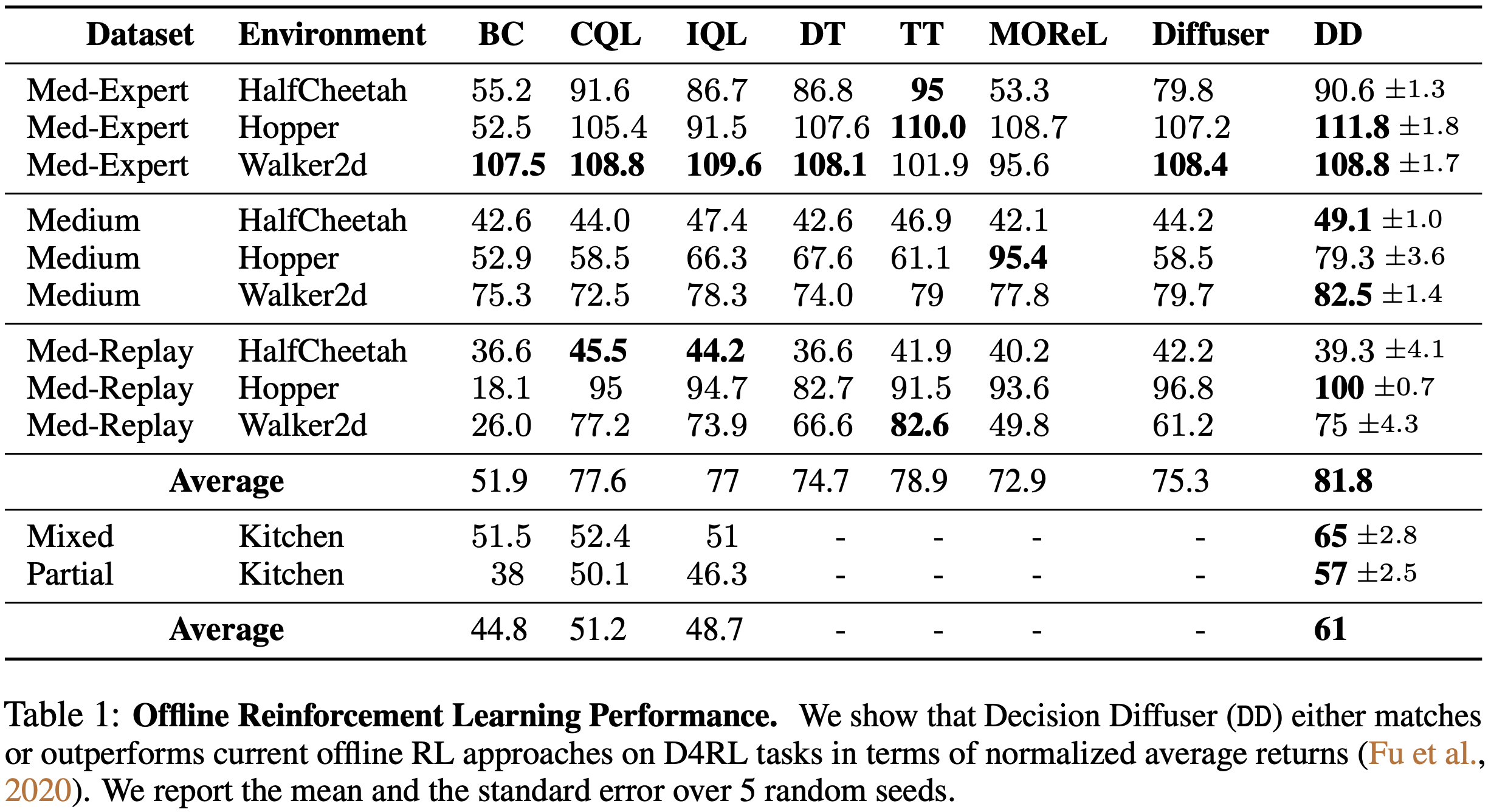
最大化回报(与强化学习方法对照)

  • 实验结论:

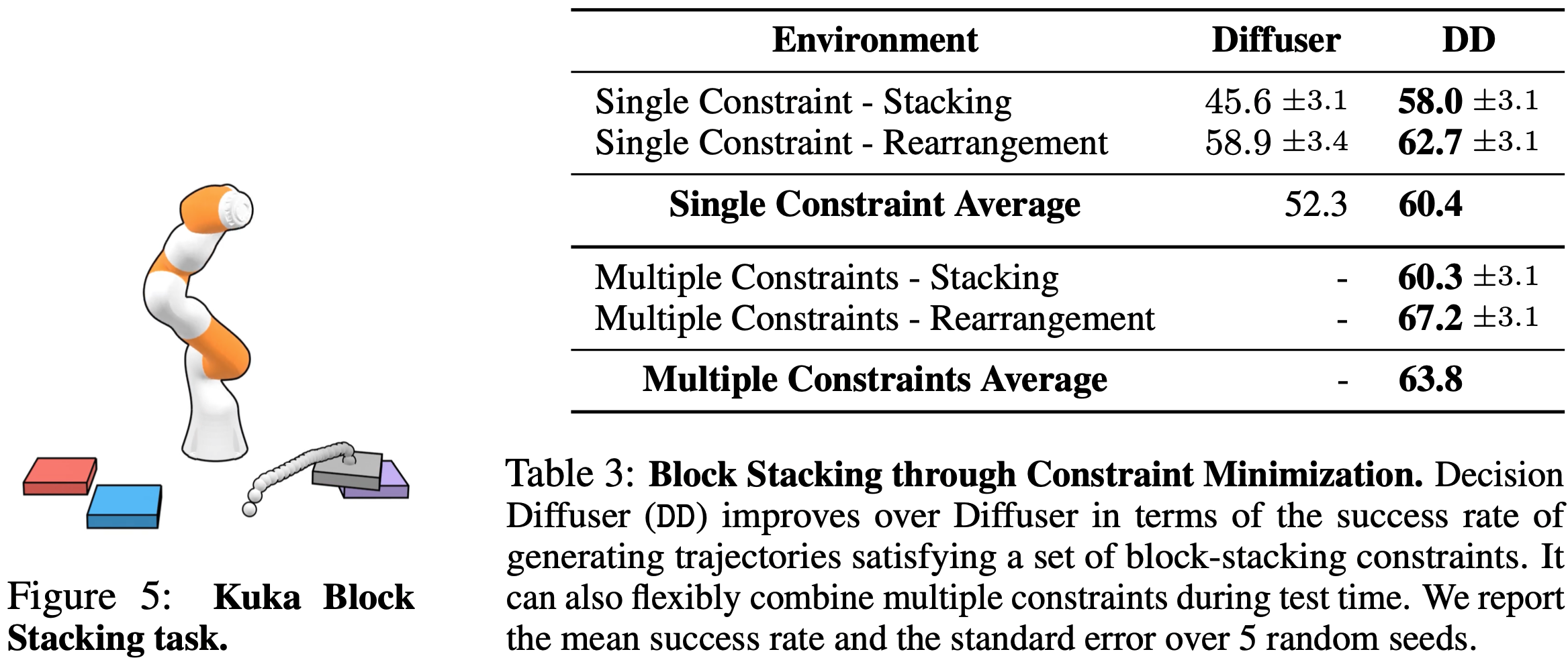
约束达成实验

  • 实验设置
    • 背景:在环境中采样轨迹数据,每个轨迹满足一个约束
    • 测试目标:
      • Single Constraint:满足任意单一约束(数据集中存在的)
      • Multiple Constraints:同时满足一些约束组合(这些组合是训练数据中没有的)
  • 实验结论

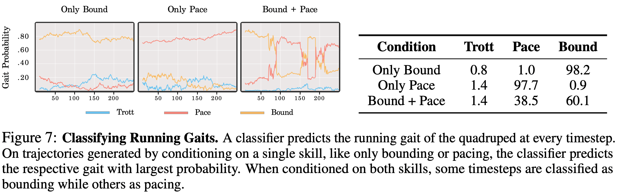
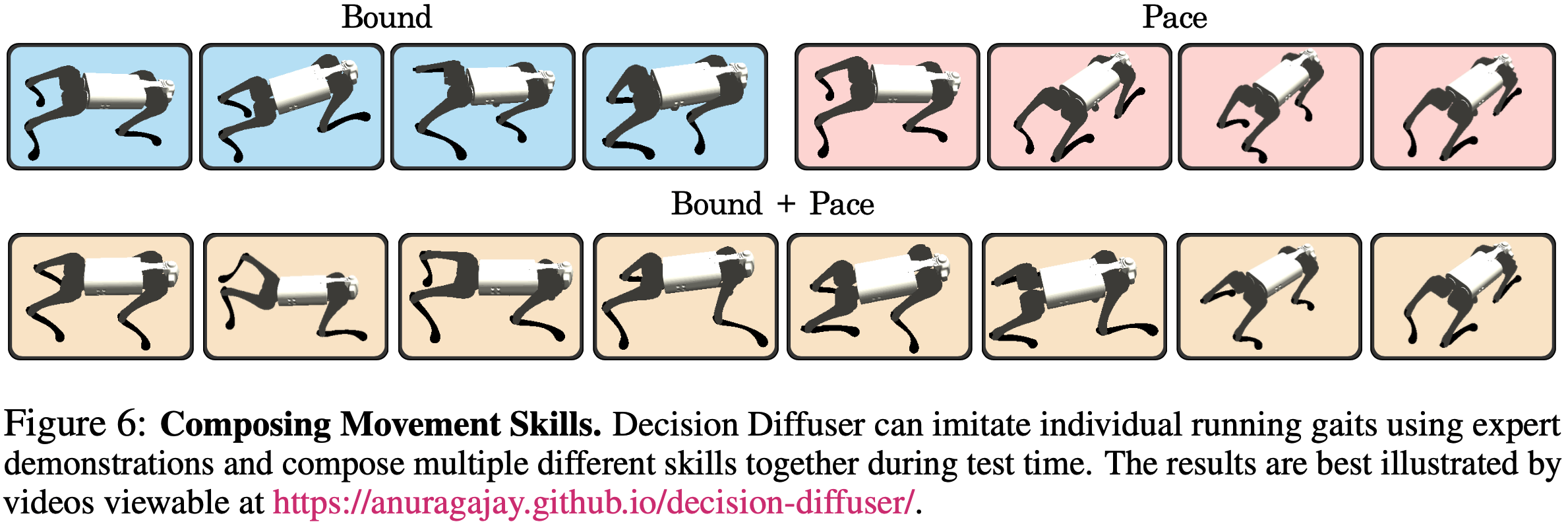
组合技能

  • 实验设置
    • 在数据集中收集包含单一技能的轨迹,然后让机器人学习各种步态,如跳跃 (bounding) 、踱步 (pacing) 和小跑 (trotting)
    • 采样时,要求机器人能按照组合步态执行运动
  • 实验结果

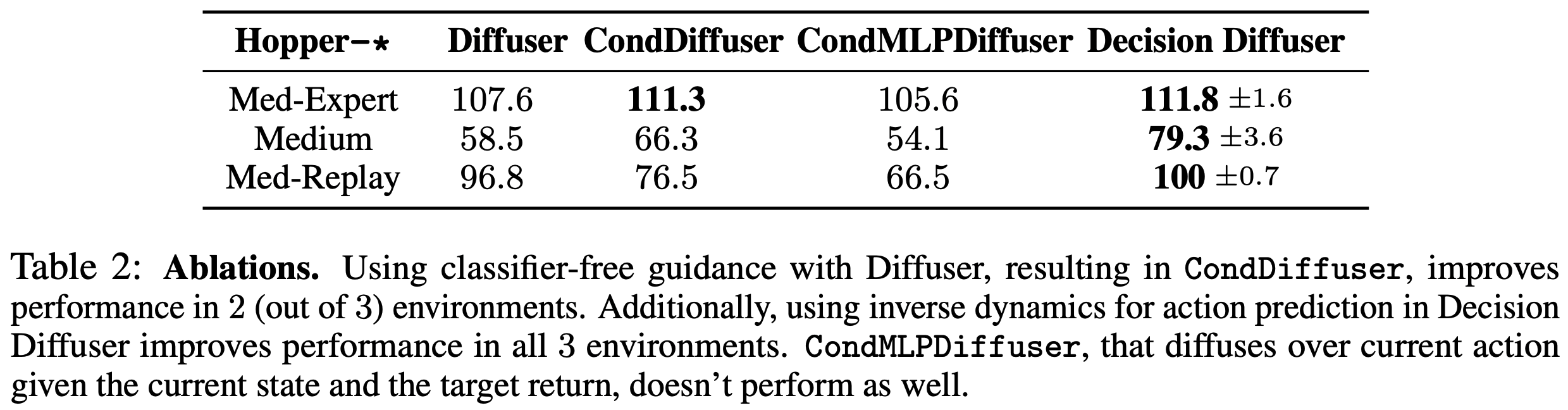
消融实验

  • 实验设置:

    • CondDiffuser :与 Diffuser 完全一致(轨迹同时纳入了状态和动作),但是没有使用 classifier guidance 而是 classifier-free guidance,输出动作不通过逆向动力学模型,而是由扩散模型去噪得到

      we also compare with the baseline CondDiffuser, which diffuses over both state and action sequences as in Diffuser without classifier-guidance

    • CondMLPDiffuser :根据state和target return来去噪生成动作(TODO问题:这个实验设置是想验证什么?target return是如何生成的?)

      We also compare against CondMLPDiffuser, a policy where the current action is denoised according to a diffusion process conditioned on both the state and return

  • 实验结论

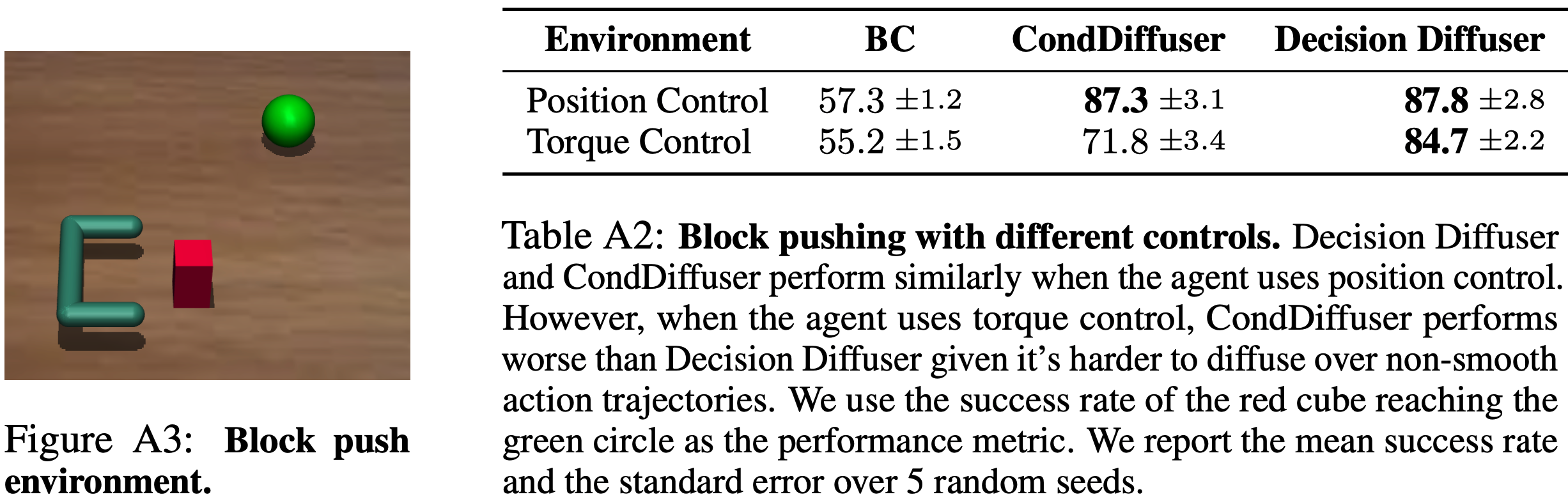
  • 补充实验(回答为什么不直接通过Diffusion生成动作,而是在已知状态 \((s,s’)\) 的情况预测动作)

    • 实验结果:
    • 在位姿控制(position control)模式下,CondDiffuser 和 Decision Diffuser 的性能差不多;
    • 在扭矩控制(torque control)模式下,Decision Diffuser 表现明显优于 CondDiffuser
    • 总结来说:较为平滑的动作可以直接使用Diffusion生成,但是对于不平滑的动作,建议使用逆向动力学模型来建模动作

超参数设置

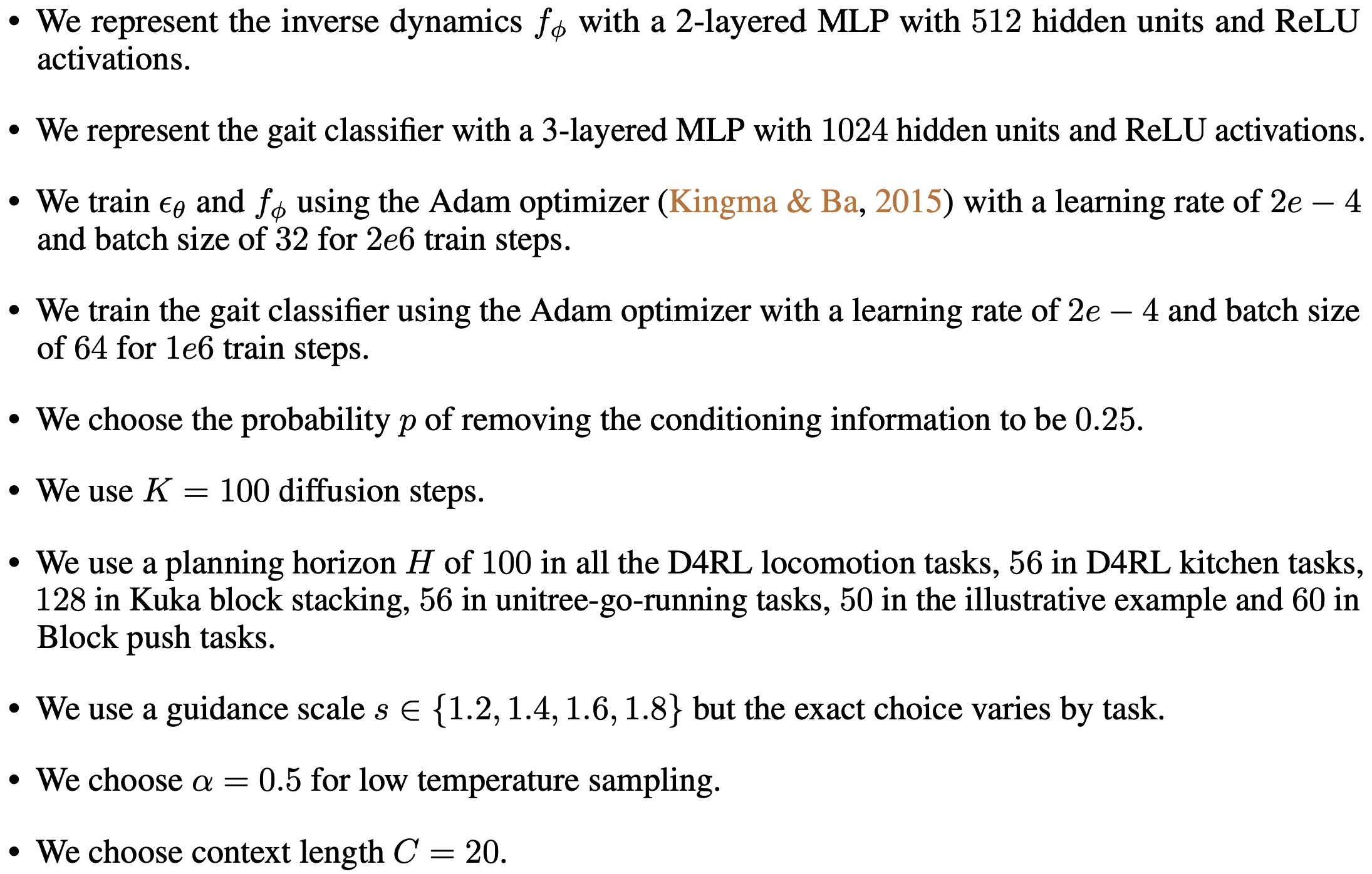
  • 超参数设置如下(From Is Conditional Generative Modeling all you need for Decision-Making?, MIT, ICLR 2023附录B)

附录:关于Guidance scale的讨论

  • Decision Diffuser使用的是Classifier-free Guidance方法,但是 \(\bar{\epsilon}_\theta(x_t, y, t)\) 的计算与原始论文Classifier-Free Diffusion Guidance, Google Research, Brain team, 2022对不齐
    • 一个说明:AIGB论文写的使用的w=0.2,但代码使用的1.2,Decision-Diffusion论文写的guidance scale s=1.2,代码使用的w=1.2
  • 在论文Classifier-Free Diffusion Guidance中,下面的 \(w\) 我们称为 \(w_\text{cdf}\):
    $$
    \begin{aligned}
    \bar{\boldsymbol{\epsilon}}_\theta(\mathbf{x}_t, t, y)
    &= \color{red}{\boldsymbol{\epsilon}_\theta(\mathbf{x}_t, t, y)} + \color{red}{w} \big(\boldsymbol{\epsilon}_\theta(\mathbf{x}_t, t, y) - \boldsymbol{\epsilon}_\theta(\mathbf{x}_t, t) \big) \\
    &= (w+1) \boldsymbol{\epsilon}_\theta(\mathbf{x}_t, t, y) - w \boldsymbol{\epsilon}_\theta(\mathbf{x}_t, t)
    \end{aligned}
    $$
  • 在Decision Diffuser中,下面的 \(w\) 我们称为 \(w_\text{dd}\),实际上,论文GLIDE也使用的这种表达:
    $$\hat{\epsilon} = \color{red}{\epsilon_\theta(\boldsymbol{x}_k(\tau), k)} + \color{red}{w}(\epsilon_\theta(\boldsymbol{x}_k(\tau),\boldsymbol{y}, k) - \epsilon_\theta(\boldsymbol{x}_k(\tau), k))$$
  • 两者的表达式不同,但是本质上,通过调整他们的 guidance scale \(w\) 可以得到相同结论,具体地,可以证明,当 \(w_\text{cfd} = w_\text{dd} - 1\) 时,两者等价
    $$
    \begin{aligned}
    \epsilon(y) + w_\text{cdf}(\epsilon(y)-\epsilon) &= \epsilon(y) + (w_\text{dd} - 1)(\epsilon(y)-\epsilon) \\
    &= \epsilon(y) + w_\text{dd} \epsilon(y) - \epsilon(y) - w_\text{dd} \epsilon + \epsilon \\
    &= \epsilon + w_1(\epsilon(y)-\epsilon)
    \end{aligned}
    $$
  • 实际应用时,Classifier-Free Diffusion Guidance中 \(w_\text{cdf} > 0\) 即可,而Decision Diffuser 和论文GLIDE中要求 \(w_\text{dd} > 1.0\) 即可
    • Decision Diffuser原始论文中未见到 \(w_\text{dd} > 1.0\) 的表达,但是附录B中有超参数 guidance scale \(s \in \{1.2,1.4,1.6,1.8\}\) 这样的表达 (注意,这里的 \(s=w\) 论文中常常混淆使用)
    • 论文GLIDE中则明确有 guidance scale \(s \ge 1.0\) 的表达 (注意,这里的 \(s=w\) 论文中常常混淆使用)
  • Decision Diffuser这种用法有一个好处,可以通过不同Diffusion误差函数相加实现满足多个条件 \(\epsilon_\theta(\boldsymbol{x}_k(\tau),\boldsymbol{y}^i(\tau), k)\) 的采样形式
    $$\hat{\epsilon} := \epsilon_\theta(\boldsymbol{x}_k(\tau),\varnothing, k) + \omega \sum_{i=1}^n (\epsilon_\theta(\boldsymbol{x}_k(\tau),\boldsymbol{y}^i(\tau), k) - \epsilon_\theta(\boldsymbol{x}_k(\tau), \varnothing, k))$$

附录:多条件组合的证明

  • 证明过程如下(From Is Conditional Generative Modeling all you need for Decision-Making?, MIT, ICLR 2023附录D):

条件为空和不满足约束都为 0?

  • 在论文中提到条件为空时,去隐向量为0,不满足约束时也是置为0,如果条件为空或者不满足约束都取0值,那么两者会混淆吧,如何理解这种情况?
  • 理解:
    • 使用 one-hot 来编码时,除非所有约束都不满足才会取值为0,不满足约束的情况和条件为空的情况本质上都是无约束的情况,所以两者等价?
1…108109110…352
San Ye

San Ye

Stay Hungry. Stay Foolish.

704 posts
53 tags
© 2026 San Ye
Powered by Hexo
|
Theme — NexT.Gemini v5.1.4