DL——VAE

• 参考文献：
  • 原始论文：Auto-Encoding Variational Bayes：

---

VAE整体说明

• 变分自编码器（Variational Auto-Encoder，VAE）是一种生成式模型，在机器学习和深度学习领域有广泛应用

---

VAE的问题设定

• 给定观测数据 \( \mathbf{x} \)，假设其由隐变量 \( \mathbf{z} \) 生成，联合分布为 \( p_\theta(\mathbf{x}, \mathbf{z}) = p_\theta(\mathbf{x}|\mathbf{z}) p(\mathbf{z}) \)，其中：
  • \( p(\mathbf{z}) \) 是隐变量的先验分布（通常为标准正态 \( \mathcal{N}(0, I) \)）
  • \( p_\theta(\mathbf{x}|\mathbf{z}) \) 是生成模型（解码器），参数为 \( \theta \)
• 目标：最大化观测数据的边际似然 \( p_\theta(\mathbf{x}) = \int p_\theta(\mathbf{x}|\mathbf{z}) p(\mathbf{z}) d\mathbf{z} \)，但积分难计算

---

一些设想（基本推导思路，可以跳过）

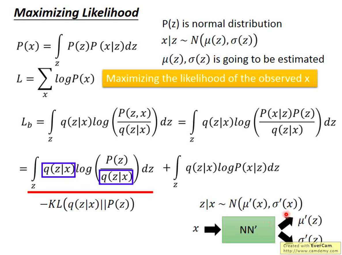
• 为了最大化概率 \(\sum_{x}\log P(x)\)，可先进行如下推导：
  $$
  \begin{align}
  L&=\sum_{x}\log P(x)\\
  &=\int_{z}q(z|x)\cdot\log P(x)dz\\
  &=\int_{z}q(z|x)\cdot\log\left(\frac{p(z,x)}{p(z|x)}\right)dz\\
  &=\int_{z}q(z|x)\cdot\log\left(\frac{p(z,x)}{q(z|x)}\cdot\frac{q(z|x)}{p(z|x)}\right)dz\\
  &=\int_{z}q(z|x)\cdot\log\left(\frac{p(z,x)}{q(z|x)}\right)dz+\underbrace{\int_{z}q(z|x)\cdot\log\left(\frac{q(z|x)}{p(z|x)}\right)dz}_{KL(q(z|x)||p(z|x))\geq0}\\
  &\geq\int_{z}q(z|x)\cdot\log\left(\frac{p(z,x)}{q(z|x)}\right)dz\\
  &=\int_{z}q(z|x)\cdot\log\left(\frac{p(x|z)\cdot p(z)}{q(z|x)}\right)dz\\
  &=\underbrace{\int_{z}q(z|x)\cdot\log(p(x|z))dz}_{Entropy}+\underbrace{\int_{z}q(z|x)\cdot\log\left(\frac{p(z)}{q(z|x)}\right)dz}_{-KL(q(z|x)||p(z))}
  \end{align}
  $$
  • 上述推导说明，最大化似然函数 \(L = \sum_{x}\log P(x)\) 可变成最大化:
    $$L’ = \int_{z}q(z|x)\cdot\log(p(x|z))dz + \int_{z}q(z|x)\cdot\log\left(\frac{p(z)}{q(z|x)}\right)dz$$
    • 实际上，后续会提到 \(L’\) 就是 \(L\) 的变分下界

---

VAE的推导

• 引入变分分布 \( q_\phi(\mathbf{z}|\mathbf{x}) \)（编码器），近似真实后验 \( p_\theta(\mathbf{z}|\mathbf{x}) \)，参数为 \( \phi \)。通过最小化 \( q_\phi(\mathbf{z}|\mathbf{x}) \) 与 \( p_\theta(\mathbf{z}|\mathbf{x}) \) 的KL散度：
  $$
  \min_{\phi} D_{\text{KL} }\left(q_\phi(\mathbf{z}|\mathbf{x}) | p_\theta(\mathbf{z}|\mathbf{x})\right)
  $$
• 展开KL散度：
  $$
  D_{\text{KL} }\left(q_\phi(\mathbf{z}|\mathbf{x}) | p_\theta(\mathbf{z}|\mathbf{x})\right) = \mathbb{E}_{q_\phi(\mathbf{z}|\mathbf{x})} \left[ \log q_\phi(\mathbf{z}|\mathbf{x}) - \log p_\theta(\mathbf{z}|\mathbf{x}) \right]
  $$
• 利用贝叶斯公式 \( p_\theta(\mathbf{z}|\mathbf{x}) = \frac{p_\theta(\mathbf{x}|\mathbf{z}) p(\mathbf{z})}{p_\theta(\mathbf{x})} \)，代入得：
  $$
  D_{\text{KL} }\left(q_\phi(\mathbf{z}|\mathbf{x}) | p_\theta(\mathbf{z}|\mathbf{x})\right) = \mathbb{E}_{q_\phi(\mathbf{z}|\mathbf{x})} \left[ \log q_\phi(\mathbf{z}|\mathbf{x}) - \log p_\theta(\mathbf{x}|\mathbf{z}) - \log p(\mathbf{z}) \right] + \log p_\theta(\mathbf{x})
  $$
• 整理后得到：
  $$
  \log p_\theta(\mathbf{x}) - D_{\text{KL} }\left(q_\phi(\mathbf{z}|\mathbf{x}) | p_\theta(\mathbf{z}|\mathbf{x})\right) = \mathbb{E}_{q_\phi(\mathbf{z}|\mathbf{x})} \left[ \log p_\theta(\mathbf{x}|\mathbf{z}) \right] - D_{\text{KL} }\left(q_\phi(\mathbf{z}|\mathbf{x}) | p(\mathbf{z})\right)
  $$

证据下界（ELBO）

• 证据下界（Evidence Lower Bound, ELBO），也称为变分下界（Variational Lower Bound, VLB）
• 由于 \( D_{\text{KL} } \geq 0 \)，有：
  $$
  \log p_\theta(\mathbf{x}) \geq \underbrace{\mathbb{E}_{q_\phi} \left[ \log p_\theta(\mathbf{x}|\mathbf{z}) \right] - D_{\text{KL} }\left(q_\phi(\mathbf{z}|\mathbf{x}) | p(\mathbf{z})\right)}_{\text{ELBO}(\theta, \phi)}
  $$
• 目标转为最大化ELBO：
  $$
  \mathcal{L}(\theta, \phi; \mathbf{x}) = \mathbb{E}_{q_\phi(\mathbf{z}|\mathbf{x})} \left[ \log p_\theta(\mathbf{x}|\mathbf{z}) \right] - D_{\text{KL} }\left(q_\phi(\mathbf{z}|\mathbf{x}) | p(\mathbf{z})\right)
  $$
  • 此时，最大化ELBO \(\mathcal{L}(\theta, \phi; \mathbf{x})\) 就可以实现最大化原始对数似然函数目标 \(\log p_\theta(\mathbf{x})\)
  • ELBO的更多等价形式见附录

损失函数分解（ELBO包含两项）

• 1. 重构项（Reconstruction Term）最大化 ：
  $$
  \mathbb{E}_{q_\phi(\mathbf{z}|\mathbf{x})} \left[ \log p_\theta(\mathbf{x}|\mathbf{z}) \right]
  $$

  • 作用：鼓励解码器重建输入数据，通常用均方误差（MSE）或交叉熵实现
  • 理解：最大化\(\mathbb{E}_{q_\phi(\mathbf{z}|\mathbf{x})} \left[ \log p_\theta(\mathbf{x}|\mathbf{z}) \right]\)等价于上面的公式等价于:
    • 从原始数据集 \(\mathcal{D}\) 任意采样一个数据 \(\mathbf{x}_0\);
    • 经过编码器 \(q_\phi(\mathbf{z}|\mathbf{x})\) 将 \(\mathbf{x}_0\) 编码成 \(\mathbf{z}\)，其中 \(\mathbf{z} \sim q_\phi(\mathbf{z}|\mathbf{x}_0)\);
    • 再经过解码器 \(p_\theta(\mathbf{x}|\mathbf{z})\) 将编码器的输出 \(\mathbf{z}\) 解码成 \(\mathbf{x}_i\)
    • 最大化 \(\log p_\theta(\mathbf{x}|\mathbf{z})\)，等价于最小化 \(\mathbf{x}_i\) 和 \(\mathbf{x}_0\) 的距离（常用交叉熵损失或者MSE）

• 2. 正则项（KL Divergence Term）最小化 ：
  $$
  D_{\text{KL} }\left(q_\phi(\mathbf{z}|\mathbf{x}) | p(\mathbf{z})\right)
  $$

  • 作用：约束编码器输出接近先验分布 \( p(\mathbf{z}) \)，避免过拟合
  • 理解：先验分布 \( p(\mathbf{z}) \)可以设定为任意我们方便采样的值，比如VAE中将其设定为标准正态分布 \(\mathcal{N}(0, I) \)

KL散度的闭式解

• 假设 \( p(\mathbf{z}) = \mathcal{N}(0, I) \)，且 \( q_\phi(\mathbf{z}|\mathbf{x}) = \mathcal{N}(\mu_\phi(\mathbf{x}), \sigma_\phi^2(\mathbf{x}) I) \)，则KL散度有闭式解：
  $$
  D_{\text{KL} }\left(q_\phi(\mathbf{z}|\mathbf{x}) | p(\mathbf{z})\right) = -\frac{1}{2} \sum_{j=1}^J \left(1 + \log \sigma_j^2 - \mu_j^2 - \sigma_j^2\right)
  $$
  • 其中 \( J \) 是隐变量维度
  • 证明过程见附录

重参数化技巧（Reparameterization Trick）

• 为可微分地采样 \( \mathbf{z} \sim q_\phi(\mathbf{z}|\mathbf{x}) \)，令：
  $$
  \mathbf{z} = \mu_\phi(\mathbf{x}) + \sigma_\phi(\mathbf{x}) \odot \epsilon, \quad \epsilon \sim \mathcal{N}(0, I)
  $$
  • 使得梯度可回传

最终损失函数（负 ELBO）

• 总损失函数 ：
  $$
  \mathcal{L}_{\text{VAE} }(\theta, \phi; \mathbf{x}) = \underbrace{\mathbb{E}_{q_\phi(\mathbf{z}|\mathbf{x})} \left[ -\log p_\theta(\mathbf{x}|\mathbf{z}) \right]}_{\text{Reconstruction Loss} } + \underbrace{D_{\text{KL} }\left(q_\phi(\mathbf{z}|\mathbf{x}) | p(\mathbf{z})\right)}_{\text{KL Divergence} }
  $$
  • 重构损失采用 MSE 或交叉熵损失函数：
    $$
    \text{Reconstruction Loss} = |\mathbf{x} - \text{Decoder}(\text{Encoder}(\mathbf{x}))|_2^2
    $$
  • KL 散度闭式解（假设 \( q_\phi(\mathbf{z}|\mathbf{x}) = \mathcal{N}(\mu, \sigma^2) \)）：
    $$
    D_{\text{KL} }\left(q_\phi(\mathbf{z}|\mathbf{x}) | p(\mathbf{z})\right) = - \frac{1}{2} \sum_{j=1}^J \left( 1 + \log \sigma_j^2 - \mu_j^2 - \sigma_j^2 \right)
    $$
    • 其中 \( J \) 是隐变量维度
• 最终，VAE的最终版MSE版损失函数为：
  $$
  \begin{align}
  \mathcal{L}_{\text{VAE} }(\theta, \phi; \mathbf{x}) &= \text{Reconstruction Loss} + D_{\text{KL} }\left(q_\phi(\mathbf{z}|\mathbf{x}) | p(\mathbf{z})\right) \\
  &= |\mathbf{x} - \text{Decoder}(\text{Encoder}(\mathbf{x}))|_2^2 - \frac{1}{2} \sum_{j=1}^J \left( 1 + \log \sigma_j^2 - \mu_j^2 - \sigma_j^2 \right)
  \end{align}
  $$
• 总体来说：VAE通过最大化ELBO，同时优化生成模型 \( p_\theta(\mathbf{x}|\mathbf{z}) \) 和推断模型 \( q_\phi(\mathbf{z}|\mathbf{x}) \)，平衡了数据重建与隐变量正则化

---

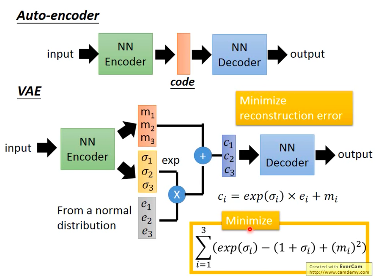
VAE网络结构

• 下面的网络输出对数方差（能保证方差非负），但是仍然使用 \(\sigma\)，容易让人误解，此时使用 \(e^\sigma\) 表示方差，此时有 \(\sigma\) 就是对数方差（原\(\log \sigma^2\)）

---

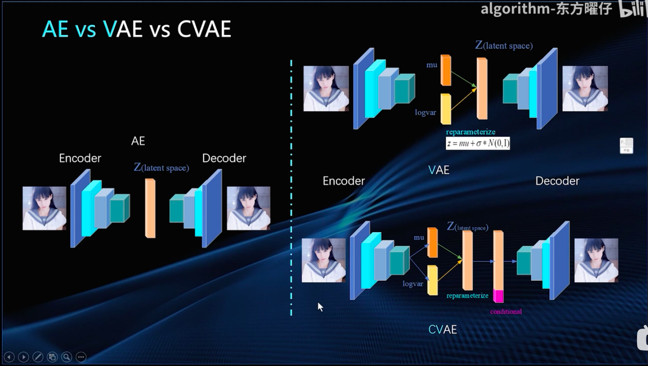
AE-VAE-CVAE

• AE-VAE-CVAE结构差异：

---

VAE的简单代码实现

• 代码实现如下：

  import torch
  import torch.nn as nn
  import torch.optim as optim
  from torchvision import datasets, transforms
  import torchvision.utils as vutils
  import matplotlib.pyplot as plt
  
  # 定义 VAE 模型
  class VAE(nn.Module):
  	def __init__(self, input_size, hidden_size=400, latent_size=20):
  		super(VAE, self).__init__()
  
  		# 编码器
  		self.fc1 = nn.Linear(input_size, hidden_size)
  		self.fc_mu = nn.Linear(hidden_size, latent_size)
  		self.fc_logvar = nn.Linear(hidden_size, latent_size)
  
  		# 解码器
  		self.fc2 = nn.Linear(latent_size, hidden_size)
  		self.fc3 = nn.Linear(hidden_size, input_size)
  
  	def encode(self, x):
  		h = torch.relu(self.fc1(x))
  		return self.fc_mu(h), self.fc_logvar(h)
  
  	def reparameterize(self, mu, logvar):
  		std = torch.exp(0.5 * logvar)
  		eps = torch.randn_like(std)
  		return mu + eps * std
  
  	def decode(self, z):
  		h = torch.relu(self.fc2(z))
  		return torch.sigmoid(self.fc3(h))
  
  	def forward(self, x):
  		mu, logvar = self.encode(x.view(-1, 784))
  		z = self.reparameterize(mu, logvar)
  		return self.decode(z), mu, logvar
  
  
  # 定义损失函数
  def loss_function(recon_x, x, mu, logvar):
  	BCE = nn.functional.binary_cross_entropy(recon_x, x.view(-1, 784), reduction='sum')
  	KLD = -0.5 * torch.sum(1 + logvar - mu.pow(2) - logvar.exp())
  	return BCE + KLD
  
  
  # 训练函数
  def train(model, train_loader, optimizer, epoch):
  	model.train()
  	train_loss = 0
  	for batch_idx, (data, _) in enumerate(train_loader):
  		data = data.to(device)
  		optimizer.zero_grad()
  		recon_batch, mu, logvar = model(data)
  		loss = loss_function(recon_batch, data, mu, logvar)
  		loss.backward()
  		train_loss += loss.item()
  		optimizer.step()
  	print(f'====> Epoch: {epoch} Average loss: {train_loss / len(train_loader.dataset):.4f}')
  
  
  # 生成图片函数
  def generate_image(model, device):
  	model.eval()
  	with torch.no_grad():
  		z = torch.randn(1, 20).to(device)
  		sample = model.decode(z).cpu()
  		sample = sample.view(1, 1, 28, 28)
  		vutils.save_image(sample, 'generated_image.png')
  		plt.imshow(sample.squeeze().numpy(), cmap='gray')
  		plt.show()
  
  
  # 数据加载
  transform = transforms.Compose([
  	transforms.ToTensor()
  ])
  train_dataset = datasets.MNIST(root='./data', train=True, transform=transform, download=True)
  train_loader = torch.utils.data.DataLoader(train_dataset, batch_size=128, shuffle=True)
  
  # 设备配置
  device = torch.device("cuda" if torch.cuda.is_available() else "cpu")
  
  # 初始化模型、优化器
  model = VAE(input_size=784).to(device)
  optimizer = optim.Adam(model.parameters(), lr=1e-3)
  
  # 训练模型
  num_epochs = 10
  for epoch in range(1, num_epochs + 1):
  	train(model, train_loader, optimizer, epoch)
  
  # 生成图片
  generate_image(model, device)

---

附录：VAE李宏毅公式推导

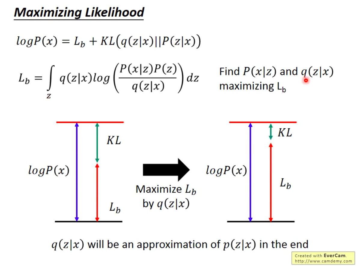
• 目标是让似然函数最大化，也就是最大化 \(\sum_x \log P(x)\)，推导可得相当于最大化变分下界(Evidence Lower Bound， \(ELBO(q)\))
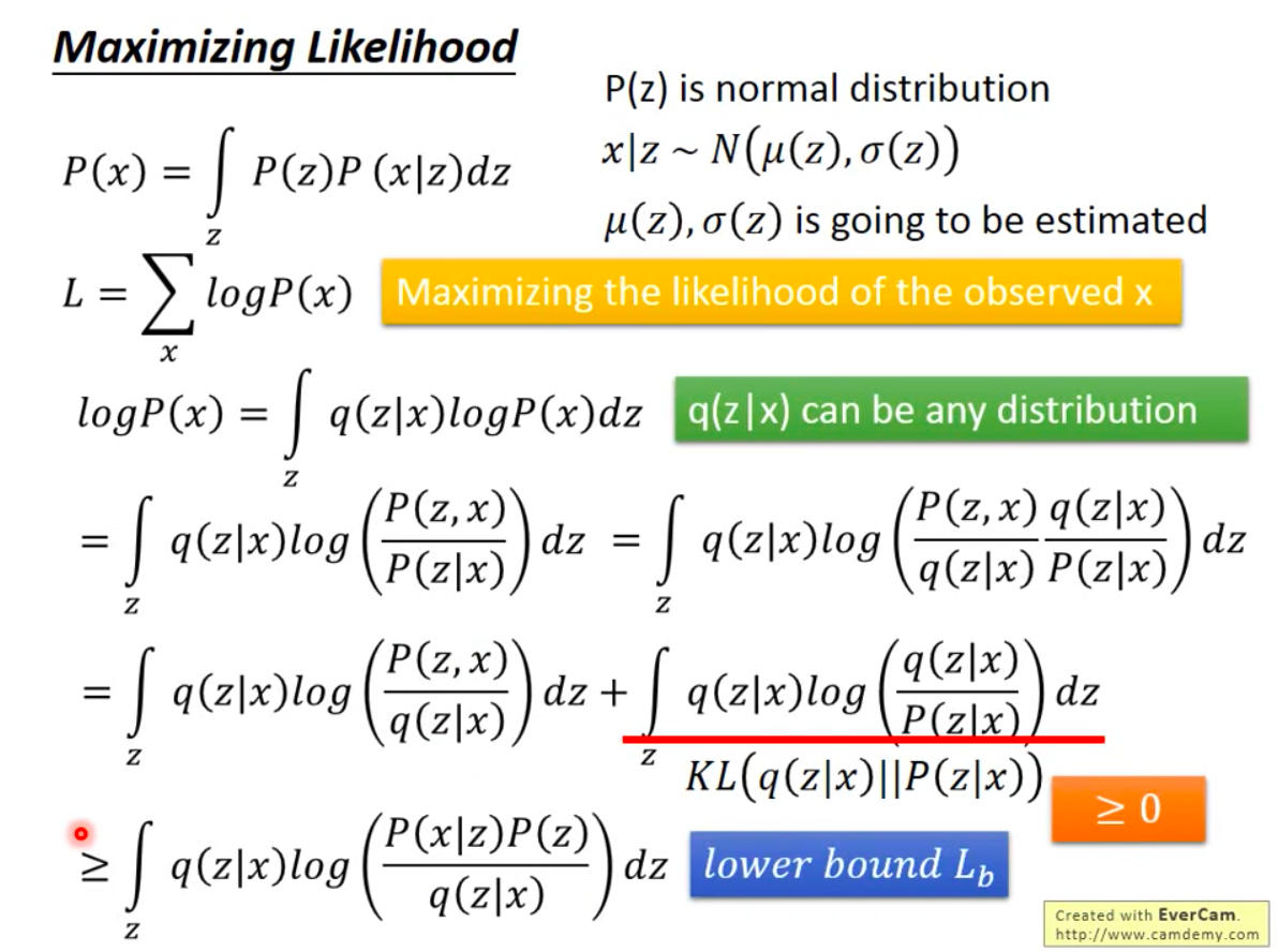
• 为什么要通过求解 \(q\) 来实现似然函数最大化/ELBO最大化呢？因为优化 \(q\) 时，与 \(P(x)\) 无关，相当于最小化KL散度
• 进一步拆解变分下界
• 变分下界的两个部分分别可用在网络中建模，两个损失函数同时优化就是VAE 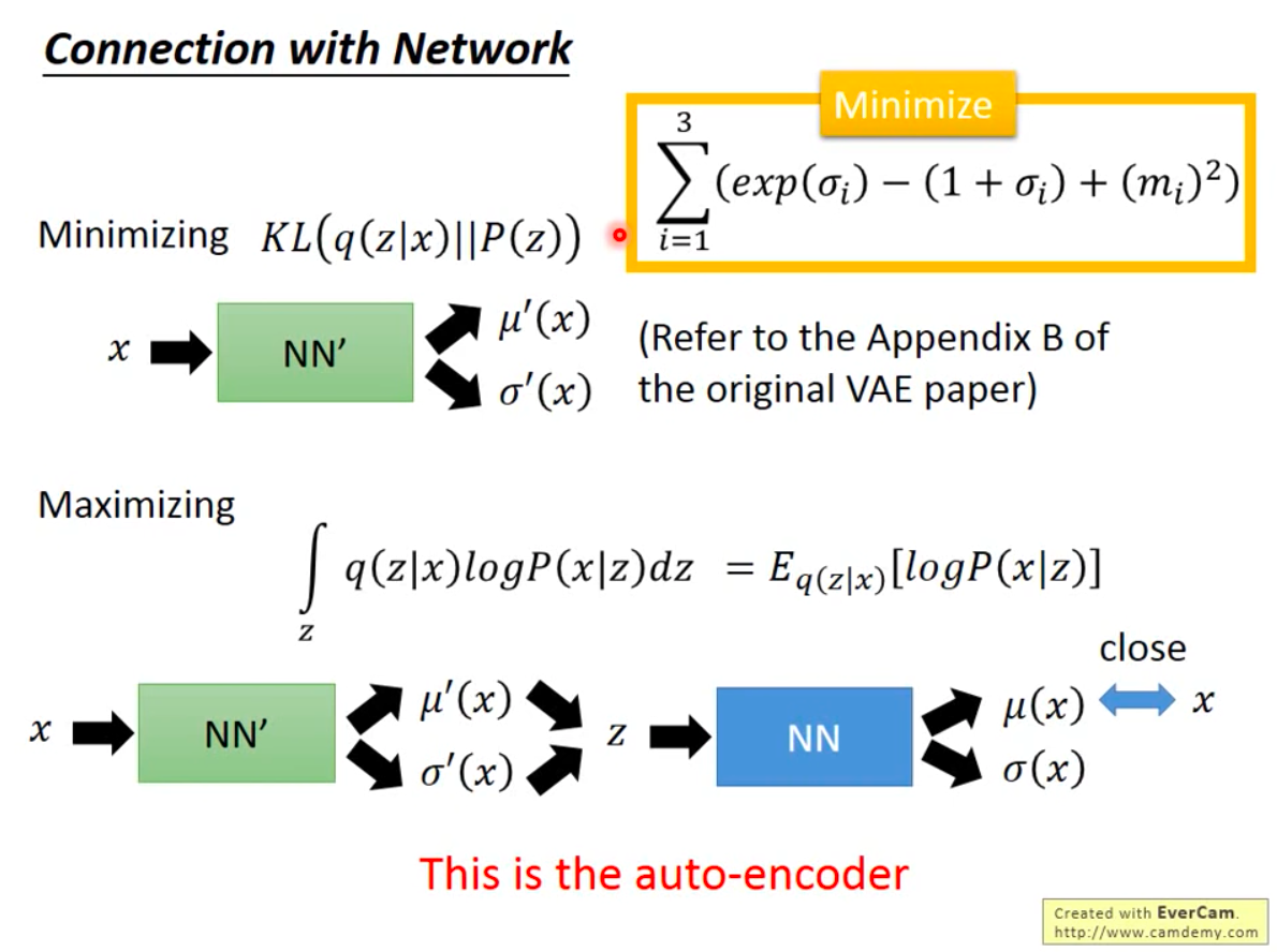* 期望部分：通过带采样的Auto-Encoder实现，损失函数为Auto-Encoder的损失函数

---

附录：KL散度闭市解的推导

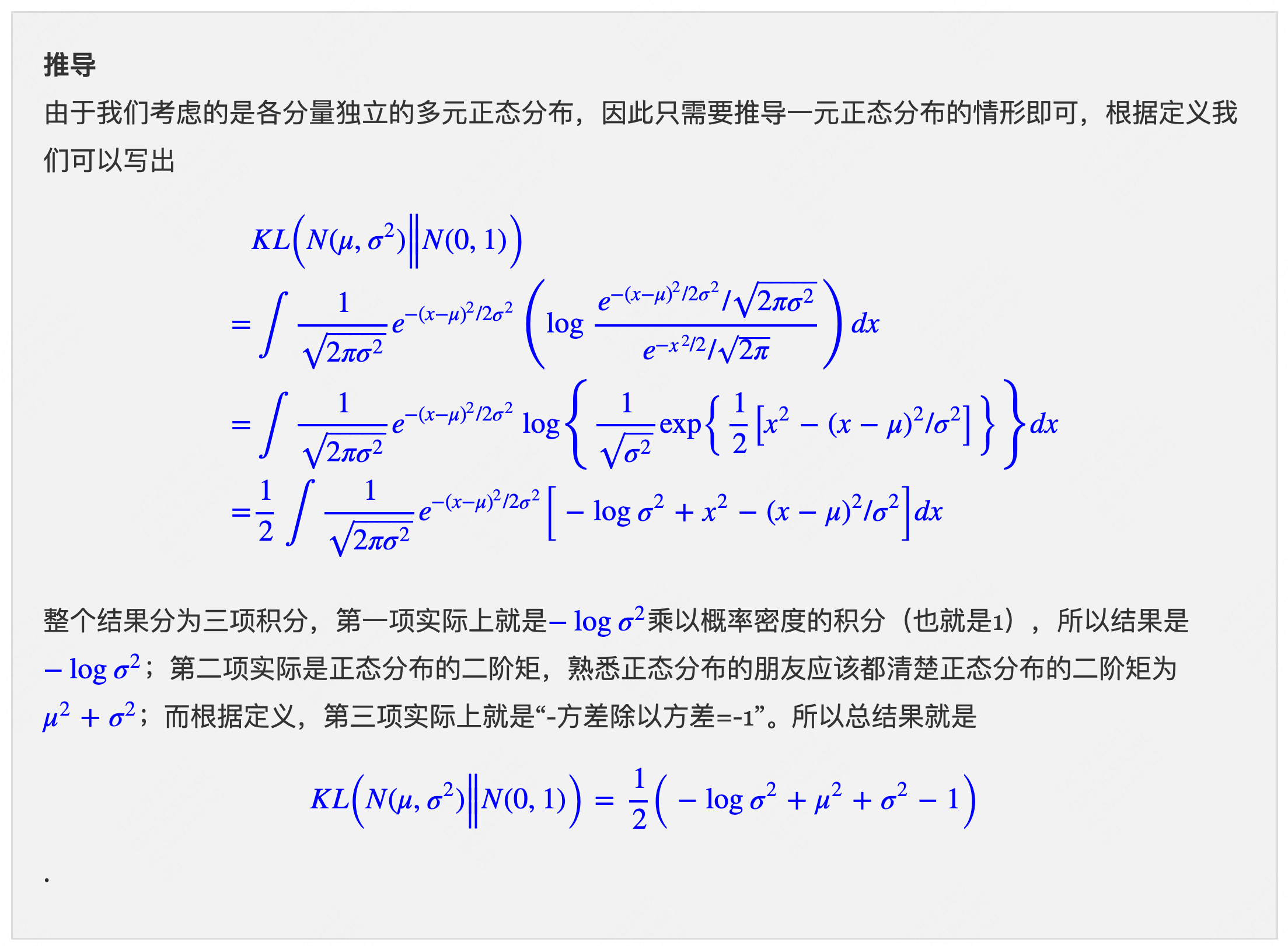
• 假设 \(p(z)\) 是均值为0方差为1的标准正太分布 \(N(0,I)\)，所以这里KL散度本质是要尽量保证分布 \(q(z|x)\) 尽可能接近标准正太分布，使用一个关于均值和方差的损失函数可以实现
• KL散度部分的闭市解推导，来自 苏神的科学空间：
• 原始论文推导可见：Auto-Encoding Variational Bayes：

---

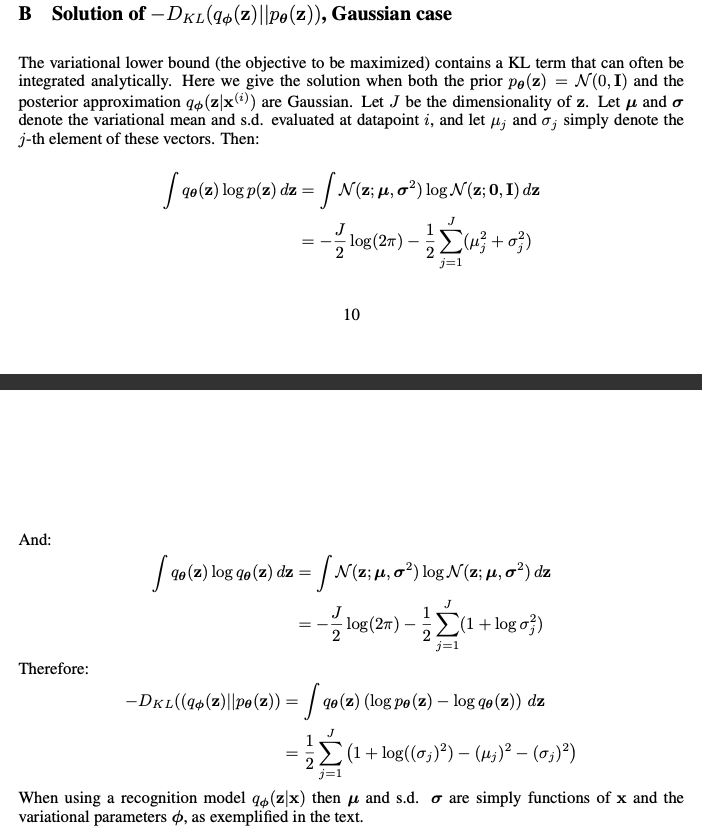
附录：ELBO的各种等价形式

• 一些等价形式：一些推导中会涉及到ELBO的不同形式：
  $$
  \begin{align}
  \mathcal{L}(\theta, \phi; \mathbf{x}) &= \mathbb{E}_{q_\phi(\mathbf{z}|\mathbf{x})} \left[ \log p_\theta(\mathbf{x}|\mathbf{z}) \right] - D_{\text{KL} }\left(q_\phi(\mathbf{z}|\mathbf{x}) | p(\mathbf{z})\right) \\
  &= \mathbb{E}_{q_\phi(\mathbf{z}|\mathbf{x})} \left[ \log p_\theta(\mathbf{x}|\mathbf{z}) \right] - \mathbb{E}_{q_\phi(\mathbf{z}|\mathbf{x})}\left[\frac{\log q_\phi(\mathbf{z}|\mathbf{x})}{\log p(\mathbf{z})}\right] \\
  &= \mathbb{E}_{q_\phi(\mathbf{z}|\mathbf{x})} \left[ \log p_\theta(\mathbf{x}|\mathbf{z}) \frac{\log p(\mathbf{z})}{\log q_\phi(\mathbf{z}|\mathbf{x})}\right] \\
  &= \mathbb{E}_{q_\phi(\mathbf{z}|\mathbf{x})} \left[ \log p_\theta(\mathbf{x}|\mathbf{z}) \frac{\log p(\mathbf{z})}{\log q_\phi(\mathbf{z}|\mathbf{x})}\right] \\
  &= \mathbb{E}_{q_\phi(\mathbf{z}|\mathbf{x})} \left[ \frac{\log p_\theta(\mathbf{x},\mathbf{z})}{\log q_\phi(\mathbf{z}|\mathbf{x})}\right] \\
  \end{align}
  $$