NLP——旋转位置编码-RoPE

• 参考链接:
  • 原始论文：(RoPE) RoFormer: Enhanced Transformer with Rotary Position Embedding, Arxiv 2023 & Neurocomputing 2024, 追一科技
  • 苏神博客：Transformer升级之路：2、博采众长的旋转式位置编码
  • 旋转式位置编码 (RoPE) 知识总结 - Soaring的文章 - 知乎，一篇把知识串的比较好的博客

---

原始 Transformer

基本 Attention 公式

• 在标准的Transformer模型中，自注意力机制（Self-Attention）的公式是核心组成部分
• 给定查询矩阵 \( Q \)、键矩阵 \( K \) 和值矩阵 \( V \)，注意力输出计算为：
  $$
  \text{Attention}(Q, K, V) = \text{softmax}\left(\frac{QK^\top}{\sqrt{d_k} }\right)V
  $$
  • \( Q \in \mathbb{R}^{n \times d_k} \), \( K \in \mathbb{R}^{m \times d_k} \), \( V \in \mathbb{R}^{m \times d_v} \)（\( n \)是目标序列长度，\( m \)是源序列长度）
  • \( d_k \) 是键/查询向量的维度
  • \( \sqrt{d_k} \) 用于缩放点积，防止梯度消失

Multi-Head Attention

• Transformer使用多头注意力扩展基本注意力：
  $$
  \text{MultiHead}(Q, K, V) = \text{Concat}(\text{head}_1, \dots, \text{head}_h)W^O
  $$
• 每个头的计算为：
  $$
  \text{head}_i = \text{Attention}(QW_i^Q, KW_i^K, VW_i^V)
  $$
  • \( W_i^Q \in \mathbb{R}^{d_{\text{model} } \times d_k} \), \( W_i^K \in \mathbb{R}^{d_{\text{model} } \times d_k} \), \( W_i^V \in \mathbb{R}^{d_{\text{model} } \times d_v} \)
  • \( W^O \in \mathbb{R}^{hd_v \times d_{\text{model} } } \) 是输出投影矩阵
  • \( h \) 是头的数量，通常满足 \( d_k = d_v = \frac{d_{\text{model} } }{h} \)

加入位置编码（仅修改输入即可）

• 在Transformer中，输入会加上正弦位置编码 \( P \in \mathbb{R}^{d_{\text{model}}} \):
  $$
  X = \text{Embedding}(x) + P
  $$
  • 其中 \( P \in \mathbb{R}^{d_{\text{model}}} \) 的每个元素为：
    $$
    P_{pos, 2i} = \sin\left(\frac{pos}{10000^{2i/d_{\text{model} } } }\right), \quad
    P_{pos, 2i+1} = \cos\left(\frac{pos}{10000^{2i/d_{\text{model} } } }\right)
    $$

Self-Attention 完整公式（以单头为例）

• 对于一个输入序列 \( X \in \mathbb{R}^{n \times d_{\text{model} } } \)：
  $$
  \begin{aligned}
  Q &= XW^Q, \quad K = XW^K, \quad V = XW^V \\
  \text{Attention}(X) &= \text{softmax}\left(\frac{QK^\top}{\sqrt{d_k} } + M\right)V
  \end{aligned}
  $$
  • \( M \) 是可选的掩码矩阵（如解码器的因果掩码）
  • 注：实际实现时，也可以直接在进入 Softmax 操作前，将 \(\frac{QK^\top}{\sqrt{d_k} }\) 的结果置为最小值 \(-e^9\)，效果是等价的

Self-Attention 简单实现

• Self-Attention的Python代码简单实现

  # 单头Attention
  class ScaledDotProductAttention(nn.Module):
      def__init__(self, d_k):
          super().__init__()
          self.d_k = d_k
  
      def forward(self, Q, K, V, mask=None):
          # Q, K, V shape: (batch_size, seq_len, d_k(or d_v))
          scores = torch.matmul(Q, K.transpose(-2, -1)) / (self.d_k ** 0.5)
          if mask is not None:
              scores = scores.masked_fill(mask == 0, -1e9)
          attn_weights = F.softmax(scores, dim=-1)
          output = torch.matmul(attn_weights, V)
          return output
  # 多头Attention
  class MultiHeadAttention(nn.Module):
      def __init__(self, d_model, num_heads):
          super().__init__()
          assert d_model % num_heads == 0, "d_model must be divisible by num_heads"
          
          self.d_model = d_model
          self.num_heads = num_heads
          self.d_k = d_model // num_heads
          
          self.W_q = nn.Linear(d_model, d_model)
          self.W_k = nn.Linear(d_model, d_model)
          self.W_v = nn.Linear(d_model, d_model)
          self.W_o = nn.Linear(d_model, d_model)
          # 使用单头Attention
          self.attention = ScaledDotProductAttention(self.d_k)
          
      def split_heads(self, x):
          """
          x shape: (batch_size, seq_len, d_model)
          return shape: (batch_size, num_heads, seq_len, d_k)
          """
          batch_size, seq_len, _ = x.size()
          return x.view(batch_size, seq_len, self.num_heads, self.d_k).transpose(1, 2)
      
      def combine_heads(self, x):
          """
          x shape: (batch_size, num_heads, seq_len, d_k)
          return shape: (batch_size, seq_len, d_model)
          """
          batch_size, _, seq_len, _ = x.size()
          return x.transpose(1, 2).contiguous().view(batch_size, seq_len, self.d_model)
      
      def forward(self, Q, K, V, mask=None):
          Q = self.W_q(Q)
          K = self.W_k(K)
          V = self.W_v(V)
          
          Q = self.split_heads(Q)
          K = self.split_heads(K)
          V = self.split_heads(V)
          
          # 如果需要，扩展mask以匹配多头（这里假设了mask是为单头准备的）
          if mask is not None:
              mask = mask.unsqueeze(1)  # (batch_size, 1, seq_len) -> (batch_size, 1, 1, seq_len)
          
          attn_output = self.attention(Q, K, V, mask)
          output = self.combine_heads(attn_output)
          output = self.W_o(output)
          return output

固定位置编码实现

• 固定位置编码，比如正弦位置编码，直接在 Attention 之前将位置编码向量加入到原始向量 \(X\) 中，Attention代码不需要做任何修改

---

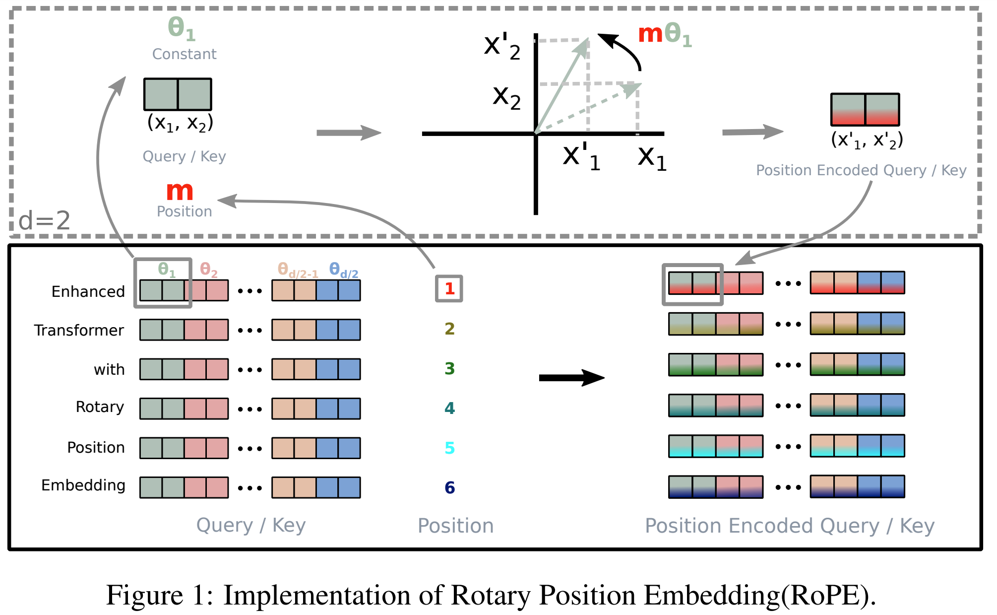
Rotary Position Embedding, RoPE

• 本节符号和原始论文 (RoPE) RoFormer: Enhanced Transformer with Rotary Position Embedding, Arxiv 2023 & Neurocomputing 2024, 追一科技 符号保持一致
• 旋转位置编码(RoPE)的核心思想 ：通过旋转矩阵将位置信息融入Self-Attention 机制中
• 基本定义 ：对于位置\( m \)的词向量\( \boldsymbol{x}_m \in \mathbb{R}^d \)，通过线性变换得到查询向量\( \boldsymbol{q}_m \)和键向量\( \boldsymbol{k}_n \)：
  $$
  \boldsymbol{q}_m = W_q \boldsymbol{x}_m, \quad \boldsymbol{k}_n = W_k \boldsymbol{x}_n
  $$
• 旋转操作 ：将\( \boldsymbol{q}_m \)和\( \boldsymbol{k}_n \)划分为\( d/2 \)个复数对（每组2维，RoPE要求维度必须是偶数，这一般都能满足），对第\( i \)组复数应用旋转矩阵：
  $$
  \begin{aligned}
  \boldsymbol{q}_m^{(i)} &= \begin{pmatrix}
  q_{m,2i} \\
  q_{m,2i+1}
  \end{pmatrix}, \quad
  \boldsymbol{k}_n^{(i)} = \begin{pmatrix}
  k_{n,2i} \\
  k_{n,2i+1}
  \end{pmatrix} \\
  R_{\theta_i}^m &= \begin{pmatrix}
  \cos m\theta_i & -\sin m\theta_i \\
  \sin m\theta_i & \cos m\theta_i
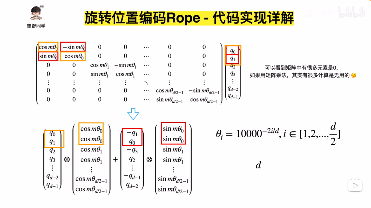
  \end{pmatrix}, \quad \theta_i = 10000^{-2i/d}
  \end{aligned}
  $$
  • 注意：位置为 \(m\) 的旋转矩阵对应正余弦角度为 \(\color{red}{m}\theta_i\)
  • 理解：旋转矩阵 \(R_{\theta_i}^m\) 可以将目标向量进行旋转，\(R_{\theta_i}^m \boldsymbol{x}\) 相当于将 \( \boldsymbol{x}\) 向逆时针方向旋转 \(m\theta_i\) 度（注意：只是旋转，并不修改原始向量的模长，因为 \(R_{\theta_i}^m\) 是正交矩阵），详情见附录
• 旋转后的向量 ：旋转后的查询和键向量为：
  $$
  \begin{aligned}
  \boldsymbol{q}_m’ = \bigoplus_{i=0}^{d/2-1} R_{\theta_i}^m \boldsymbol{q}_m^{(i)}, \quad
  \boldsymbol{k}_n’ = \bigoplus_{i=0}^{d/2-1} R_{\theta_i}^n \boldsymbol{k}_n^{(i)}
  \end{aligned}
  $$
  • 其中\( \oplus \)表示向量拼接：
    $$\bigoplus_{i=0}^{d/2-1} R_{\theta_i}^m \boldsymbol{q}_m^{(i)} = \text{Concat}(\{ R_{\theta_i}^m \boldsymbol{q}_m^{(i)}\}_{i=0}^{d/2-1})$$
• 旋转后的Attention权重变化
  $$
  \begin{equation}
  (\boldsymbol{\mathcal{R}}_m \boldsymbol{q}_m)^{\top}(\boldsymbol{\mathcal{R}}_n \boldsymbol{k}_n) = \boldsymbol{q}_m^{\top} \boldsymbol{\mathcal{R}}_m^{\top}\boldsymbol{\mathcal{R}}_n \boldsymbol{k}_n = \boldsymbol{q}_m^{\top} \boldsymbol{\mathcal{R}}_{n-m} \boldsymbol{k}_n
  \end{equation}
  $$
  • 位置为 \(m\) 的向量 \(\boldsymbol{q}_m\) 乘以矩阵 \(\boldsymbol{\mathcal{R}}_m\)；位置为 \(n\) 的向量 \(\boldsymbol{k}_n\) 乘以矩阵 \(\boldsymbol{\mathcal{R}}_n\)（注意角标）
  • 上面的式子中等式是恒成立的（\( \boldsymbol{\mathcal{R}}_m^{\top}\boldsymbol{\mathcal{R}}_n = \boldsymbol{\mathcal{R}}_{\color{red}{n-m}}\)的详细证明见附录），右边的 \(\boldsymbol{\mathcal{R}}_{\color{red}{n-m}}\)仅与相对位置 \(n-m\) 有关，体现了相对位置编码的核心要义
    • 注：\(\boldsymbol{\mathcal{R}}_{m-n}\) 和 \(\boldsymbol{\mathcal{R}}_{n-m}\) 不相等，旋转角度相同，但方向相反
• 展开成矩阵相乘的形式为（refer to Transformer升级之路：2、博采众长的旋转式位置编码）：
  $$
  \begin{equation}\scriptsize{\underbrace{\begin{pmatrix}
  \cos m\theta_0 & -\sin m\theta_0 & 0 & 0 & \cdots & 0 & 0 \\
  \sin m\theta_0 & \cos m\theta_0 & 0 & 0 & \cdots & 0 & 0 \\
  0 & 0 & \cos m\theta_1 & -\sin m\theta_1 & \cdots & 0 & 0 \\
  0 & 0 & \sin m\theta_1 & \cos m\theta_1 & \cdots & 0 & 0 \\
  \vdots & \vdots & \vdots & \vdots & \ddots & \vdots & \vdots \\
  0 & 0 & 0 & 0 & \cdots & \cos m\theta_{d/2-1} & -\sin m\theta_{d/2-1} \\
  0 & 0 & 0 & 0 & \cdots & \sin m\theta_{d/2-1} & \cos m\theta_{d/2-1} \\
  \end{pmatrix}}_{\boldsymbol{\mathcal{R}}_m} \begin{pmatrix}q_0 \\ q_1 \\ q_2 \\ q_3 \\ \vdots \\ q_{d-2} \\ q_{d-1}\end{pmatrix}}\end{equation}
  $$
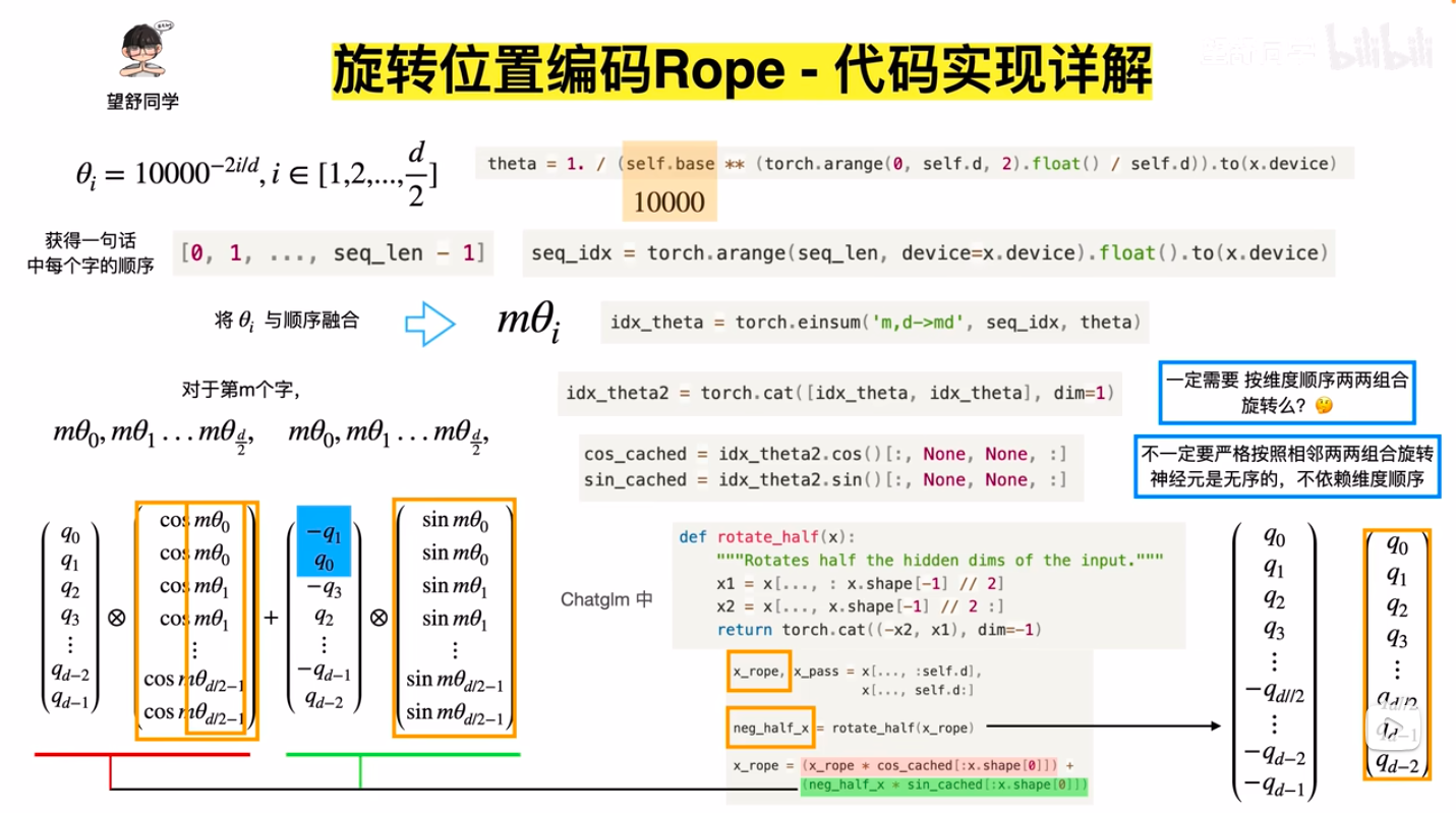
• 由于旋转矩阵是一个稀疏矩阵，所以旋转过程可以改进为如下等价实现：
  $$
  \begin{equation}\begin{pmatrix}q_0 \\ q_1 \\ q_2 \\ q_3 \\ \vdots \\ q_{d-2} \\ q_{d-1}
  \end{pmatrix}\otimes\begin{pmatrix}\cos m\theta_0 \\ \cos m\theta_0 \\ \cos m\theta_1 \\ \cos m\theta_1 \\ \vdots \\ \cos m\theta_{d/2-1} \\ \cos m\theta_{d/2-1}
  \end{pmatrix} + \begin{pmatrix}-q_1 \\ q_0 \\ -q_3 \\ q_2 \\ \vdots \\ -q_{d-1} \\ q_{d-2}
  \end{pmatrix}\otimes\begin{pmatrix}\sin m\theta_0 \\ \sin m\theta_0 \\ \sin m\theta_1 \\ \sin m\theta_1 \\ \vdots \\ \sin m\theta_{d/2-1} \\ \sin m\theta_{d/2-1}
  \end{pmatrix}\end{equation}
  $$
  • 其中 \(\otimes\) 是按位相乘
• RoPE下的Attention公式总结 ：（旋转位置编码的核心公式）
  $$
  \begin{aligned}
  \text{Attention}(\boldsymbol{x}) &= \text{softmax}\left(\frac{(\boldsymbol{q}’)^\top \boldsymbol{k}’}{\sqrt{d} }\right)V
  \end{aligned}
  $$
  • 注：\(V\) 是 Attention 中的 Value 矩阵，中不需要位置编码信息
  • 这里使用 \((\boldsymbol{q}’)^\top \boldsymbol{k}’\)，转置在 \(\boldsymbol{q}’\) 上，和原始论文表达方式一致，实际上这种表示是OK的，数学中常用这种表示 ，这种表示下，向量为列向量；原始 Transformer 论文中的符号转置在 Key 上，此时向量为行向量
• 原始论文中的RoPE示意图：

---

多头注意力下的 RoPE

• 为了跟传统的 Transformer 符号对齐，本节改用 \(Q,K,V\)表示矩阵，与 RoPE 原始论文符号不再一致
• 给定输入序列 \( X \in \mathbb{R}^{n \times d_{\text{model} } } \)，先投影到查询、键、值空间：
  $$
  Q = XW^Q, \quad K = XW^K, \quad V = XW^V
  $$
  • 其中 \( W^Q, W^K \in \mathbb{R}^{d_{\text{model} } \times d_k} \), \( W^V \in \mathbb{R}^{d_{\text{model} } \times d_v} \)
• 应用旋转位置编码（RoPE） ：对 \( Q \) 和 \( K \) 的每个位置 \( m \) 和 \( n \) 的分量应用旋转矩阵 \( R_{\theta}^m \) 和 \( R_{\theta}^n \)：
  $$
  \begin{aligned}
  Q’ &= \text{RoPE}(Q) = \bigoplus_{i=0}^{d_k/2-1} R_{\theta_i}^m Q^{(i)} \\
  K’ &= \text{RoPE}(K) = \bigoplus_{i=0}^{d_k/2-1} R_{\theta_i}^n K^{(i)}
  \end{aligned}
  $$
  • \( Q^{(i)} \in \mathbb{R}^2 \) 和 \( K^{(i)} \in \mathbb{R}^2 \) 是 \( Q \) 和 \( K \) 的第 \( i \) 个二维分量
  • \( \oplus \)表示向量拼接：
    $$\bigoplus_{i=0}^{d_k/2-1} R_{\theta_i}^m Q^{(i)} = \text{Concat}(\{R_{\theta_i}^m Q^{(i)}\}_{i=0}^{d_k/2-1} )$$
• 旋转矩阵 \( R_{\theta_i}^m \) 定义为：
  $$
  R_{\theta_i}^m = \begin{pmatrix}
  \cos m\theta_i & -\sin m\theta_i \\
  \sin m\theta_i & \cos m\theta_i
  \end{pmatrix}, \quad \theta_i = 10000^{-2i/d_k}
  $$
• 多头注意力输出
  $$
  \text{MultiHead}(Q, K, V) = \text{Concat}(\text{head}_1, \dots, \text{head}_H) W^O \\
  \text{head}_h = \text{Softmax}\left(\frac{Q^{\prime}_h {K^{\prime}_h}^\top}{\sqrt{d_k} }\right) V_h
  $$
  • 其中 \( W^O \in \mathbb{R}^{H d_v \times d_{\text{model} } } \) 是输出投影矩阵
• 多头注意力下的 RoPE 的 Attention 公式总结 :
  $$
  \begin{aligned}
  \text{Attention}(Q,K,V) &= \text{softmax}\left(\frac{(\text{RoPE}(Q))(\text{RoPE}(K))^\top}{\sqrt{d_k} }\right)V \\
  \text{where} \quad \text{RoPE}(X) &= \bigoplus_{i=0}^{d/2-1} R_{\theta_i}^m X^{(i)}
  \end{aligned}
  $$

多头注意力下的 RoPE 实现

• 多头注意力下的RoPE PyTorch 实现 (待补充)
  • 注：多头注意力下，每个头是独立编码的（每个头维度从 0 开始），且使用的旋转矩阵一样，即旋转矩阵的维度 \(d = d_{\text{head}} = d_{\text{model}}/h\)

---

关于 RoPE 的一些讨论

• RoPE 传统 Transformer 的区别 ：
  • 传统Transformer：位置编码是加性的（\( X + P \)）
  • RoPE：位置编码是乘性的（通过旋转矩阵直接修改 \( Q \) 和 \( K \)）
• 相对位置保持性 ：
  • 旋转后的注意力分数 \( [Q’ K’^\top]_{m,n} \) 仅依赖于相对位置 \( m-n \)，满足线性注意力性质
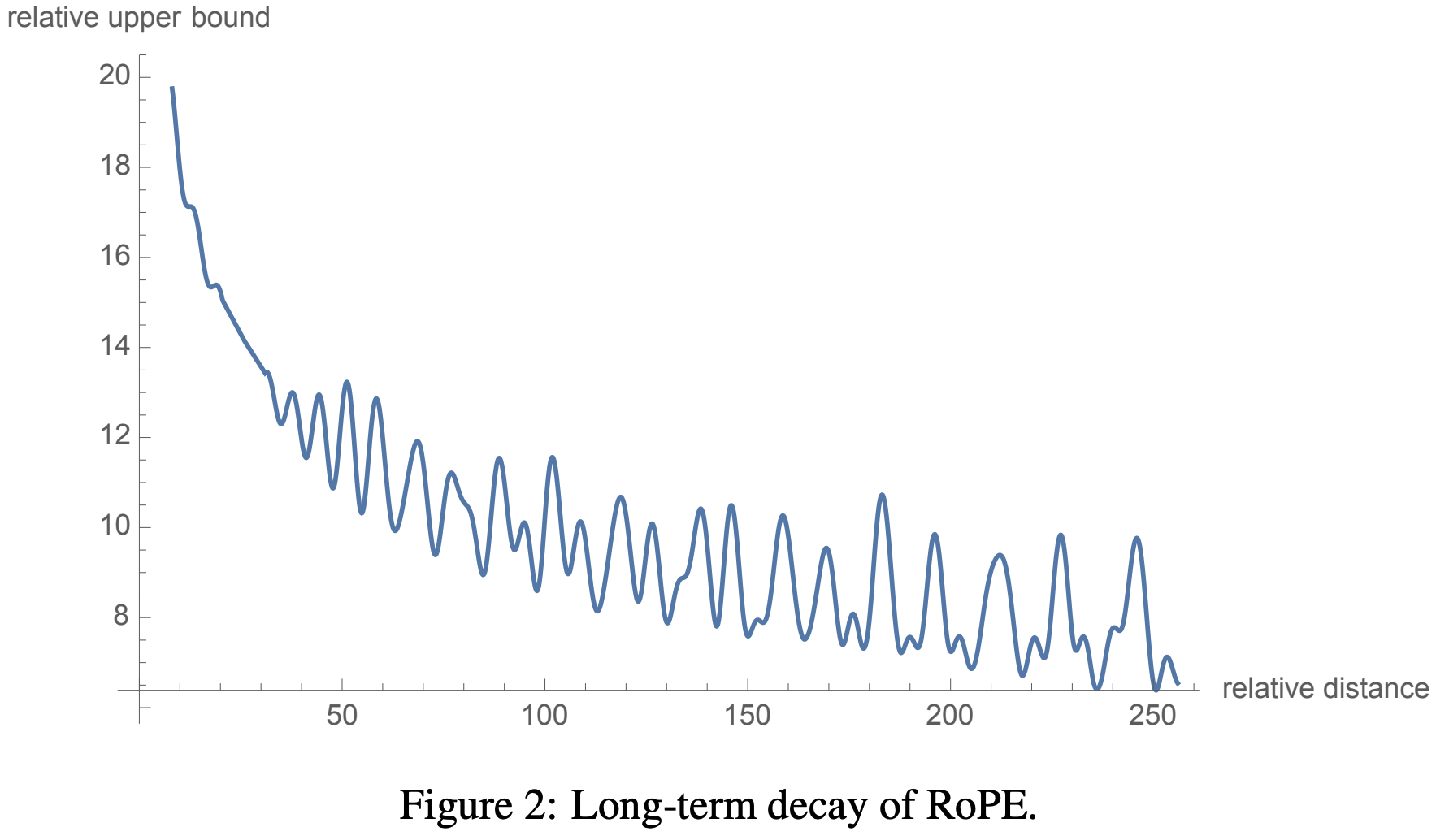
• 远程衰减性 ：（注：如下图所示的远距离衰减，会导致太远的距离下，难以区分位置，效果不好，外推性变差？）

---

附录：相对位置旋转公式证明

• 目标：证明 \( \boldsymbol{\mathcal{R}}_m^{\top}\boldsymbol{\mathcal{R}}_n = \boldsymbol{\mathcal{R}}_{\color{red}{n-m}}\)
• 考虑到 \(\boldsymbol{\mathcal{R}}_m\) 是以二维子矩阵为单位的“对角”矩阵，故只要证明 \((R_{\theta_i}^m)^\top R_{\theta_i}^n = R_{\theta_i}^{\color{red}{n-m}}\) 即可，证明过程如下：
• 给定旋转矩阵 \( R_{\theta_i}^m \) 定义为：
  $$
  R_{\theta_i}^m = \begin{pmatrix}
  \cos m\theta_i & -\sin m\theta_i \\
  \sin m\theta_i & \cos m\theta_i
  \end{pmatrix}
  $$
• 其转置矩阵为：
  $$
  (R_{\theta_i}^m)^\top = \begin{pmatrix}
  \cos m\theta_i & \sin m\theta_i \\
  -\sin m\theta_i & \cos m\theta_i
  \end{pmatrix}
  $$
• 计算 \((R_{\theta_i}^m)^\top R_{\theta_i}^n\)
  $$
  (R_{\theta_i}^m)^\top R_{\theta_i}^n = \begin{pmatrix}
  \cos m\theta_i & \sin m\theta_i \\
  -\sin m\theta_i & \cos m\theta_i
  \end{pmatrix}
  \begin{pmatrix}
  \cos n\theta_i & -\sin n\theta_i \\
  \sin n\theta_i & \cos n\theta_i
  \end{pmatrix}
  $$
• 回顾三角函数和差角公式：
  $$
  \sin(A \pm B) = \sin A \cos B \pm \cos A \sin B \\
  \cos(A \pm B) = \cos A \cos B \mp \sin A \sin B
  $$
• 计算矩阵乘积的每个元素：
  • 左上角元素：
    $$
    \begin{align}
    \cos m\theta_i \cdot \cos n\theta_i + \sin m\theta_i \cdot \sin n\theta_i &= \cos(n\theta_i - m\theta_i) \\
    &= \cos((n - m)\theta_i) \\
    \end{align}
    $$
  • 右上角元素：
    $$
    \begin{align}
    \cos m\theta_i \cdot (-\sin n\theta_i) + \sin m\theta_i \cdot \cos n\theta_i &= -\cos m\theta_i \sin n\theta_i + \sin m\theta_i \cos n\theta_i \\
    &= \sin m\theta_i \cos n\theta_i - \cos m\theta_i \sin n\theta_i\\
    & = \sin((m-n)\theta_i) \\
    & = - \sin((n-m)\theta_i)
    \end{align}
    $$
  • 左下角元素：
    $$
    \begin{align}
    -\sin m\theta_i \cdot \cos n\theta_i + \cos m\theta_i \cdot \sin n\theta_i &= -\sin m\theta_i \cos n\theta_i + \cos m\theta_i \sin n\theta_i \\
    &= \sin n\theta_i \cos m\theta_i - \cos n\theta_i \sin m\theta_i \\
    &= \sin((n - m)\theta_i)
    \end{align}
    $$
  • 右下角元素：
    $$
    \begin{align}
    -\sin m\theta_i \cdot (-\sin n\theta_i) + \cos m\theta_i \cdot \cos n\theta_i &= \sin m\theta_i \sin n\theta_i + \cos m\theta_i \cos n\theta_i \\
    &= \sin m\theta_i \sin n\theta_i + \cos m\theta_i \cos n\theta_i \\
    &= \cos((n - m)\theta_i)
    \end{align}
    $$
• 因此，乘积矩阵为：
  $$
  (R_{\theta_i}^m)^\top R_{\theta_i}^n = \begin{pmatrix}
  \cos((n - m)\theta_i) & -\sin((n - m)\theta_i) \\
  \sin((n - m)\theta_i) & \cos((n - m)\theta_i)
  \end{pmatrix} = R_{\theta_i}^{\color{red}{n-m}}
  $$
• 至此，我们证明了：
  $$
  (R_{\theta_i}^m)^\top R_{\theta_i}^n = R_{\theta_i}^{\color{red}{n-m}}
  $$
• 证毕

---

附录：不同参数下 RoPE 对 Attention 的影响

• RoPE原始论文已经说明了随着距离的增长，Attention Score 有越来越小的趋势（且长距离部分会波动）
• 下面是固定 query_index 下，Attention Score 随 key_index（横轴）变化的图像（代码参考链接修改的 旋转式位置编码 (RoPE) 知识总结 - Soaring的文章 - 知乎）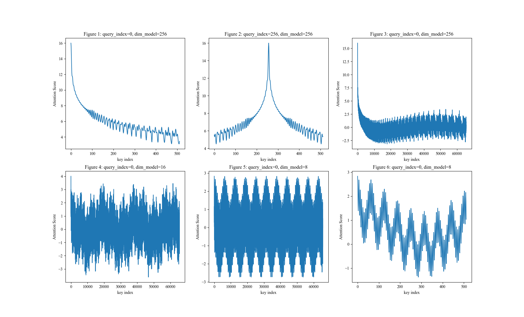
• 从上图可以观察到：
  • 图1：RoPE确实有远距离衰减趋势（震荡递减），且dim_model=256时，q,k 距离为500时Attention值已经衰减的较小了
  • 图2：与图1类似，RoPE的衰减是对称的（图2展示的是当 query_index=256时的图像）；
    • 注：注意虽然 Attention Score 是对称相等的，但是旋转角度是相反的，即 \(\boldsymbol{\mathcal{R}}_{m-n}\) 和 \(\boldsymbol{\mathcal{R}}_{n-m}\) 旋转角度相同，但方向是相反的
  • 图3：RoPE 在拉到足够长的距离后，不会一直衰减（从后续的图可以知道实际上还是周期函数，只是周期很大）
  • 图4+图5：与图1对比可以发现，RoPE 在拉到足够长的距离后，实际上还是周期函数，只不过周期与 d_model 相关（d_model越大，周期越长），图4说明了当 d_model=8 时，周期是 10000 左右
  • 图6：缩小了图5的横轴区间，将图5的前半部分图像放大了看，是在小周期上震荡的，且还存在图5所示的大周期
• 附上图的代码：
  >>>点击展开折叠内容...

  # refer to: [旋转式位置编码 (RoPE) 知识总结 - Soaring的文章 - 知乎](https://zhuanlan.zhihu.com/p/662790439)
  import numpy as np
  import matplotlib.pyplot as plt
  from matplotlib.axes import Axes
  
  def create_sin_cos_table_cache(max_num_tokens, dim_model):
      # 所有pos下对应的cos/sin值分别存储为矩阵
      theta = 10000 ** (-np.arange(0, dim_model, 2) / dim_model)
      theta = theta.reshape(-1, 1).repeat(2, axis=1).flatten()
  
      pos = np.arange(0, max_num_tokens)
      table = pos.reshape(-1, 1) @ theta.reshape(1, -1)  # [max_num_tokens, dim_model]
  
      sin_table_cache = np.sin(table)
      sin_table_cache[:, ::2] = -sin_table_cache[:, ::2]
  
      cos_table_cache = np.cos(table)
      return sin_table_cache, cos_table_cache
  
  def rotate_half(q_vec):
      # 将q_vec的值两个一组分组并在分组内对调，实现从[q_0,q_1,q_2,q_3,...,q_{d-1},q_d]到的转换[q_1,q_0,q_3,q_2,...,q_d,q_{d-1}]
      return q_vec.reshape(-1, 2)[:, ::-1].flatten()
  
  def rotary(vec, pos, sin_table, cos_table):
      # 原始论文中的公式
      return vec * cos_table[pos] + rotate_half(vec) * sin_table[pos]
  
  def plot(plt_obj: Axes, pic_index, query_index=0, dim_model=256, max_num_tokens=8192, step=1):
      # q_vec 和 k_vec 都设定为1，仅关注 RoPE 引发的Attention Score的变化
      q_vec = np.ones(dim_model)
      k_vec = np.ones(dim_model)
      sin_table, cos_table = create_sin_cos_table_cache(max_num_tokens, dim_model)
  
      rotated_q_vec = rotary(q_vec, query_index, sin_table, cos_table)
      k_indices = np.arange(0, max_num_tokens, step)
      rotated_k_vecs = rotary(k_vec, k_indices, sin_table, cos_table)
      attn_scores = (rotated_k_vecs @ rotated_q_vec) / np.sqrt(dim_model) # 未经过Softmax的Attention权重，用于展示RoPE对原始Attention Score
  
      plt_obj.plot(k_indices, attn_scores)
      plt_obj.set_title(f"Figure {pic_index}: query_index={query_index}, dim_model={dim_model}")
      plt_obj.set_xlabel("key index")
      plt_obj.set_ylabel("Attention Score")
  
  plt.rcParams.update({
      "font.sans-serif": ["Times New Roman", ],
      "font.size": 10
  })
  
  _, axes = plt.subplots(nrows=2, ncols=3, figsize=(10, 10))
  plot(axes[0, 0], 1, query_index=0, max_num_tokens=512)
  plot(axes[0, 1], 2, query_index=256, max_num_tokens=512)
  plot(axes[0, 2], 3, query_index=0, dim_model=256, max_num_tokens=65535)
  # plot(axes[1, 0], 4, query_index=0, dim_model=32, max_num_tokens=65535)
  plot(axes[1, 0], 4, query_index=0, dim_model=16, max_num_tokens=65535)
  plot(axes[1, 1], 5, query_index=0, dim_model=8, max_num_tokens=65536)
  plot(axes[1, 2], 6, query_index=0, dim_model=8, max_num_tokens=512)
  plt.show()

---

附录：如何改进 RoPE 以实现绝对位置编码？

• 当前的设计仅能实现相对位置编码（因为 Query 和 Key 的内积只与他们的相对位置有关，与绝对位置无关），但如果在 Value 上也施加位置编码则能实现绝对位置编码的能力
• 让研究人员绞尽脑汁的Transformer位置编码中苏神提到：

  这样一来，我们得到了一种融绝对位置与相对位置于一体的位置编码方案，从形式上看它有点像乘性的绝对位置编码，通过在 \(\boldsymbol{q},\boldsymbol{k}\) 中施行该位置编码，那么效果就等价于相对位置编码，而如果还需要显式的绝对位置信息，则可以同时在 \(\boldsymbol{v}\) 上也施行这种位置编码。总的来说，我们通过绝对位置的操作，可以达到绝对位置的效果，也能达到相对位置的效果

---

附录：旋转体现在哪里？

• 旋转体现在 \(\boldsymbol{q}_m\)（或\(\boldsymbol{k}_n\)） 的每两个维度组成的向量 \(\boldsymbol{q}_m^{(i)} = \begin{pmatrix} q_{m,2i} \\ q_{m,2i+1} \end{pmatrix}\) 经过 RoPE 变换前后，他们的向量长度不变，即：
  $$
  \begin{pmatrix}cos(m\theta_1) &-sin(m\theta_1) \\ sin(m\theta_1) &cos(m\theta_1)\end{pmatrix} \begin{pmatrix}q_{m,2i} \\ q_{m,2i+1}\end{pmatrix} = \begin{pmatrix}q_{m,2i}\cdot cos(m\theta_1) -q_{m,2i+1}\cdot sin(m\theta_1) \\ q_{m,2i}\cdot sin(m\theta_1)+ q_{m,2i+1}\cdot cos(m\theta_1) \end{pmatrix} \\
  $$
• 进一步，由于 \((cos(m\theta_1))^2 + (sin(m\theta_1))^2 = 1\) 有
  $$
  \begin{align}
  \left|\begin{pmatrix}q_{m,2i}\cdot cos(m\theta_1) -q_{m,2i+1}\cdot sin(m\theta_1) \\ q_{m,2i}\cdot sin(m\theta_1)+ q_{m,2i+1}\cdot cos(m\theta_1) \end{pmatrix} \right| &= \sqrt{\left(q_{m,2i}\cdot cos(m\theta_1) -q_{m,2i+1}\cdot sin(m\theta_1)\right)^2 + \left(q_{m,2i}\cdot sin(m\theta_1)+ q_{m,2i+1}\cdot cos(m\theta_1)\right)^2} \\
  &= \sqrt{(q_{m,2i})^2 + (q_{m,2i+1})^2}
  \end{align}
  $$
• 也就是说： \(\boldsymbol{q}_m\)（或\(\boldsymbol{k}_n\)）相邻两两维度在变换前后的向量长度并没有变化，是一个旋转操作

---

附录：可视化RoPE旋转过程

• 旋转矩阵 \(R_{\theta_i}^m\) 的定义如下：
  $$
  \begin{aligned}
  R_{\theta_i}^m &= \begin{pmatrix}
  \cos m\theta_i & -\sin m\theta_i \\
  \sin m\theta_i & \cos m\theta_i
  \end{pmatrix}, \quad \theta_i = 10000^{-2i/d}
  \end{aligned}
  $$
• 旋转矩阵 \(R_{\theta_i}^m\) 可以将目标向量进行旋转，\(R_{\theta_i}^m \boldsymbol{x}\) 相当于将 \( \boldsymbol{x}\) 向逆时针方向旋转 \(m\theta_i\) 度
• 当 \(m\theta_i = \frac{\pi}{4}\) 时，其旋转可视化结果如下：
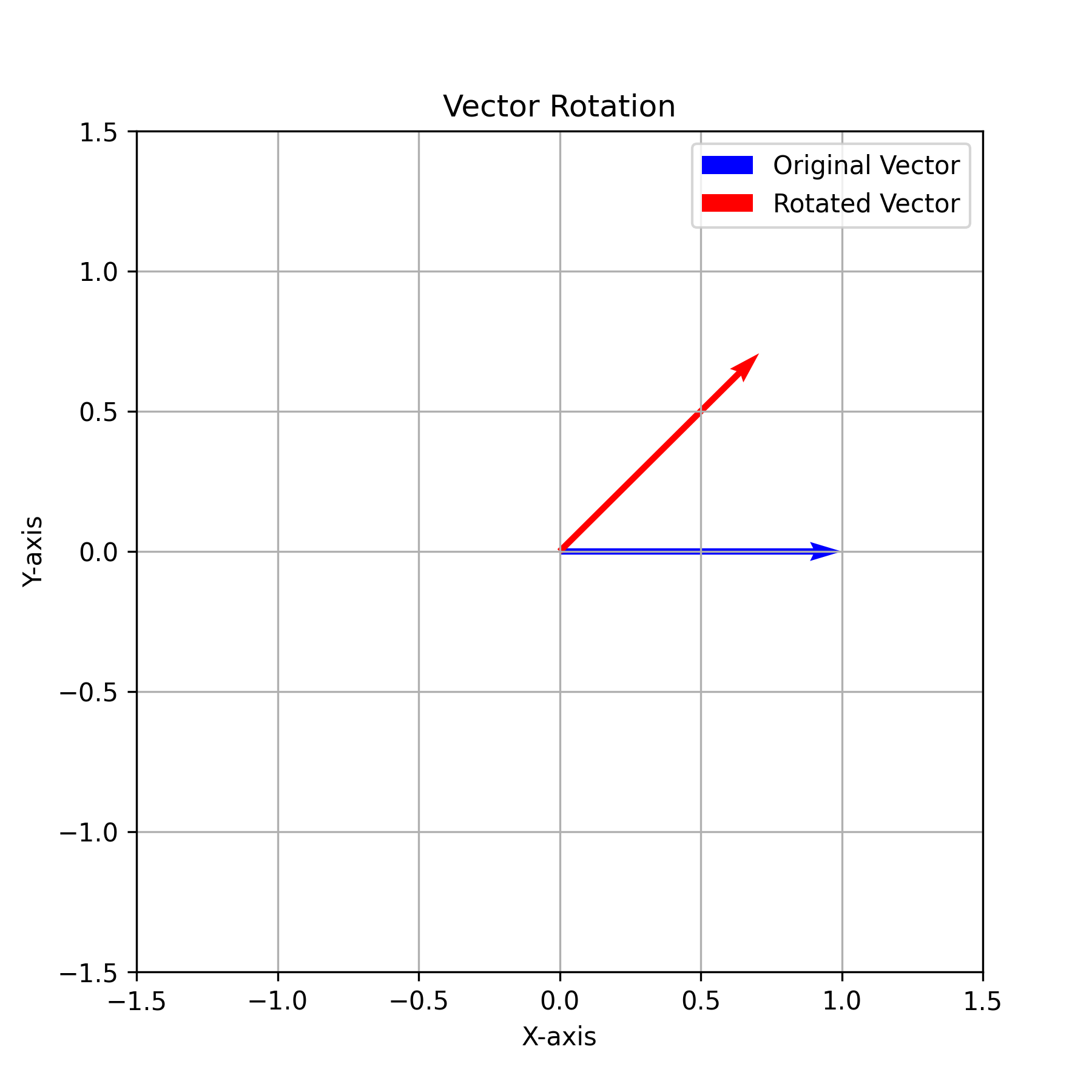
• 实现上述旋转的代码如下
  >>>点击展开折叠内容...

     import numpy as np
     import matplotlib.pyplot as plt
  
     # 设定原始向量 x
     x = np.array([1, 0])
  
     # 角度转换为弧度
     angle = np.radians(45)
  
     # 旋转矩阵定义
     R = np.array([[np.cos(angle), -np.sin(angle)],
                 [np.sin(angle), np.cos(angle)]])
  
     # 矩阵惩罚实现旋转向量
     x_rotated = R @ x
  
     plt.rcParams['figure.dpi'] = 300
  
     plt.figure(figsize=(6, 6))
     plt.quiver(0, 0, x[0], x[1], angles='xy', scale_units='xy', scale=1, color='b', label='Original Vector')
     plt.quiver(0, 0, x_rotated[0], x_rotated[1], angles='xy', scale_units='xy', scale=1, color='r', label='Rotated Vector')
  
     plt.xlim(-1.5, 1.5)
     plt.ylim(-1.5, 1.5)
  
     plt.grid(True)
  
     plt.legend()
     plt.title('Vector Rotation')
     plt.xlabel('X-axis')
     plt.ylabel('Y-axis')
  
  plt.savefig("./demo.png")
     plt.show()

---

附录：RoPE的诞生历史

• RoPE方案来自苏神原始博客:
  • 2021年2月在让研究人员绞尽脑汁的Transformer位置编码中提出想法
  • 2023年3月在Transformer升级之路：2、博采众长的旋转式位置编码中给出详细方案和推导，同时提交论文到arXiv上
  • 原始论文：Roformer: Enhanced Transformer With Rotray Position Embedding，该论文24年发表于Neurocomputing期刊上（《Neurocomputing》是国际知名期刊,被列为中科院SCI二区top期刊,CCF-C类期刊）
  • 随后，各种开源大模型开始使用RoPE，RoPE逐渐成为大模型的标配

---

附录：RoPE的高维扩展

• 论文介绍当前的是一维 RoPE，每 2 维为一组，旋转矩阵为 \(2\times 2\)，在二维 RoPE 场景中，可以每 4 维为一组，旋转矩阵变成 \(4\times 4\) 即可，详情见 旋转式位置编码 (RoPE) 知识总结
• 将四个维度作为一组:
  $$
  \boldsymbol{R}_{m_1,m_2} =
  \begin{bmatrix}
  \cos m_1 \theta & -\sin m_1 \theta & 0 & 0 \\
  \sin m_1 \theta & \cos m_1 \theta & 0 & 0 \\
  0 & 0 & \cos m_2 \theta & -\sin m_2 \theta \\
  0 & 0 & \sin m_2 \theta & \cos m_2 \theta
  \end{bmatrix}
  $$
• 上述分组下满足:
  $$
  \mathbf{R}_{m_1,m_2}^{\top} \cdot \mathbf{R}_{n_1,n_2} = \mathbf{R}_{n_1 - m_1,n_2 - m_2}
  $$
• 注：更高维度的可以继续扩展，比如三维的扩展为每 6 维为一组，旋转矩阵为 \(6\times 6\) 即可

---

附录：RoPE中的复数和旋转矩阵等价性证明

问题定义

• 定义二维旋转矩阵和向量如下：
  $$
  \begin{align}
  R_{\theta_i}^m &= \begin{pmatrix}
  \cos m\theta_i & -\sin m\theta_i \\
  \sin m\theta_i & \cos m\theta_i
  \end{pmatrix} \\
  \boldsymbol{x} &= \begin{pmatrix} x_1 \\ x_2
  \end{pmatrix}
  \end{align}
  $$
• 目标：证明下面的等式
  $$R_{\theta_i}^m \boldsymbol{x} = z e^{i m\theta_i}$$
  • 其中 \( z = x_1 + i x_2 \) 是向量 \(\boldsymbol{x} = \begin{pmatrix} x_1 \\ x_2 \end{pmatrix}\) 的复数形式
  • 即目标是证明：旋转矩阵 \( R_{\theta_i}^m \) 作用在 \(\boldsymbol{x}\) 上相当于将复数 \( z \) 乘以旋转因子 \( e^{i m\theta_i} \)

证明

• 方程左边展开
  $$
  R_{\theta_i}^m \boldsymbol{x} = \begin{pmatrix}
  \cos m\theta_i & -\sin m\theta_i \\
  \sin m\theta_i & \cos m\theta_i
  \end{pmatrix}
  \begin{pmatrix} x_1 \\ x_2 \end{pmatrix} =
  \begin{pmatrix}
  x_1 \cos m\theta_i - x_2 \sin m\theta_i \\
  x_1 \sin m\theta_i + x_2 \cos m\theta_i
  \end{pmatrix}
  $$

  • 这个结果对应的复数为：
    $$
    R_{\theta_i}^m \boldsymbol{x} = (x_1 \cos m\theta_i - x_2 \sin m\theta_i) + i (x_1 \sin m\theta_i + x_2 \cos m\theta_i)
    $$

• 等方程右边展开

  • 右边的 \(\boldsymbol{x} e^{i m\theta_i}\) 表示将复数 \( z = x_1 + i x_2 \) 乘以 \( e^{i m\theta_i} \)，即：
    $$
    z e^{i m\theta_i} = (x_1 + i x_2)(\cos m\theta_i + i \sin m\theta_i)
    $$
  • 可以重新整理为：
    $$ z e^{i m\theta_i} = (x_1 \cos m\theta_i - x_2 \sin m\theta_i) + i (x_1 \sin m\theta_i + x_2 \cos m\theta_i) $$
  • 展开后与旋转矩阵作用的结果完全一致

• 结论： 在复数表示下，旋转矩阵 \( R_{\theta_i}^m \) 作用在向量 \(\boldsymbol{x}\) 上等价于将对应的复数 \( z \) 乘以旋转因子 \( e^{i m\theta_i} \)。因此，等式成立：
  $$
  \color{red}{R_{\theta_i}^m \boldsymbol{x} = \boldsymbol{x} e^{i m\theta_i}}
  $$

---

附录：旋转位置编码的其他推导过程

• 下面的推导过程来自通俗易懂-大模型的关键技术之一：旋转位置编码rope（2）和通俗易懂-大模型的关键技术之一:旋转位置编码rope （3），推导过程看过，基本没有问题，先截图，以后有时间再手打一遍
• \(q,k\) 向量旋转后再进行Attention，注意图中 \(e^{im\theta}\) 的 \(i\) 是虚数的意思，这里使用二维向量 \((\boldsymbol{W}_q\boldsymbol{x}_m)\) 乘以一个虚数的本质是想表达向量内积的意思（虚数可以展开成二维向量），此外，\(a_{m,n}\) 表示 Attention 权重，在不考虑权重时值为 Softmax，Element-wise看：\(a_{m,n} =\frac{\exp(\frac{q^T_m k_n}{\sqrt{d_k}})}{\sum_{j=1}^N \exp(\frac{q^T_m k_j}{\sqrt{d_k}})}\)，注：下图中的表达有误，实际上应该是 \(a_{m,n}=\frac{\exp(\frac{ {x^{\prime}_m}^T x^{\prime}_n}{\sqrt{d_k} })}{\sum_{j=1}^N \exp(\frac{ {x^{\prime}_m}^T x^{\prime}_j}{\sqrt{d_k} })}\)（详情见原始论文：(RoPE) RoFormer: Enhanced Transformer with Rotary Position Embedding, Arxiv 2023 & Neurocomputing 2024, 追一科技 ）
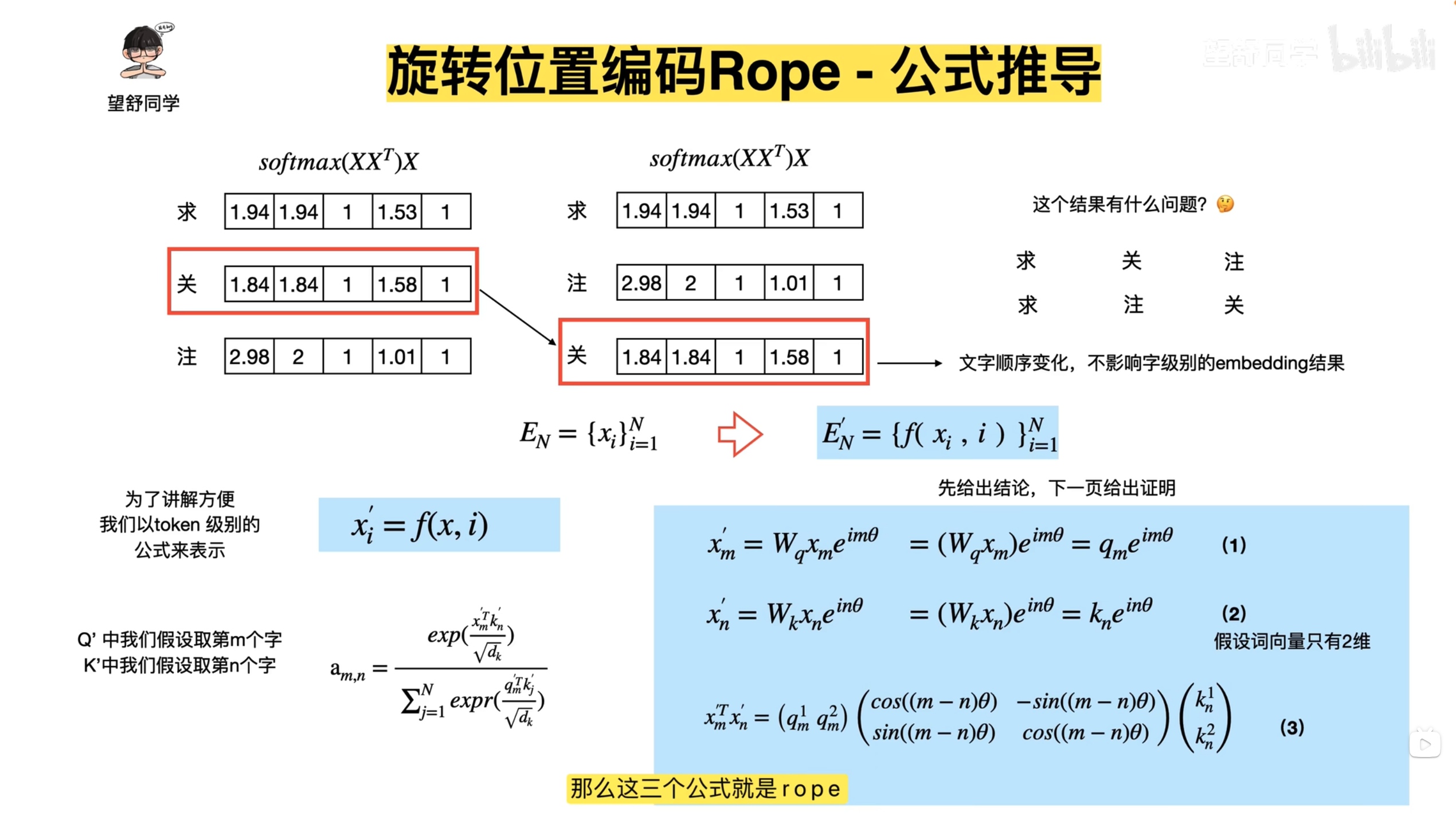
• 公式1,2，推导出公式3的过程（内积角度）
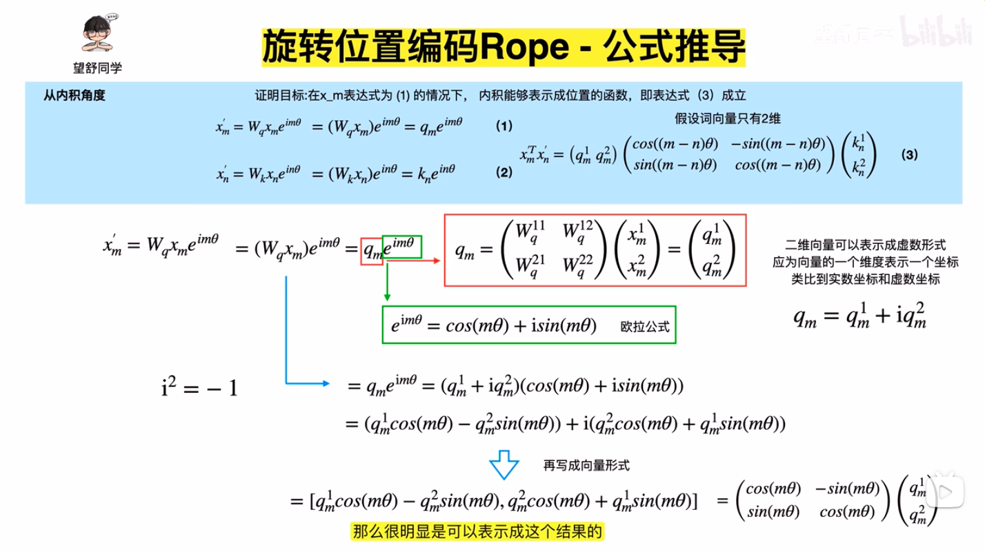
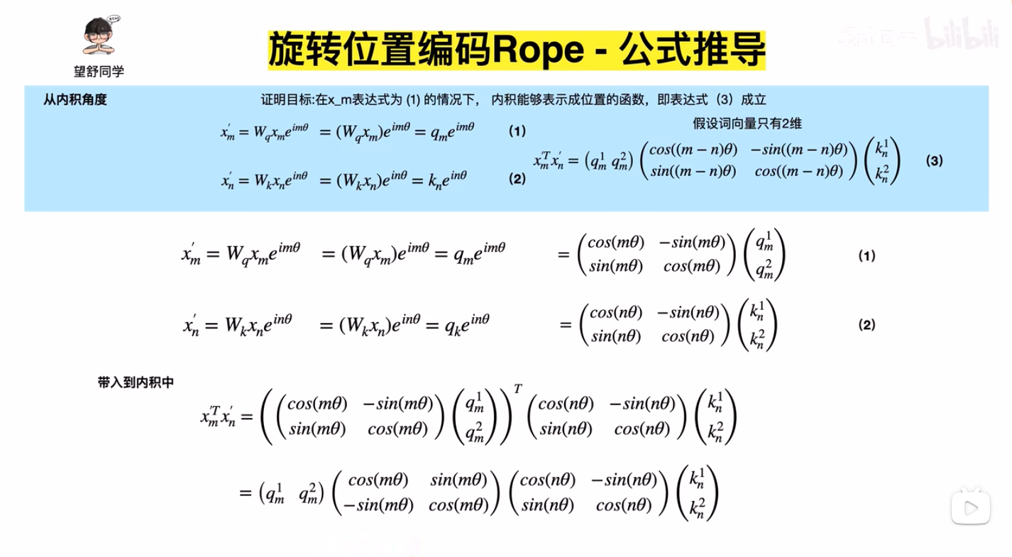
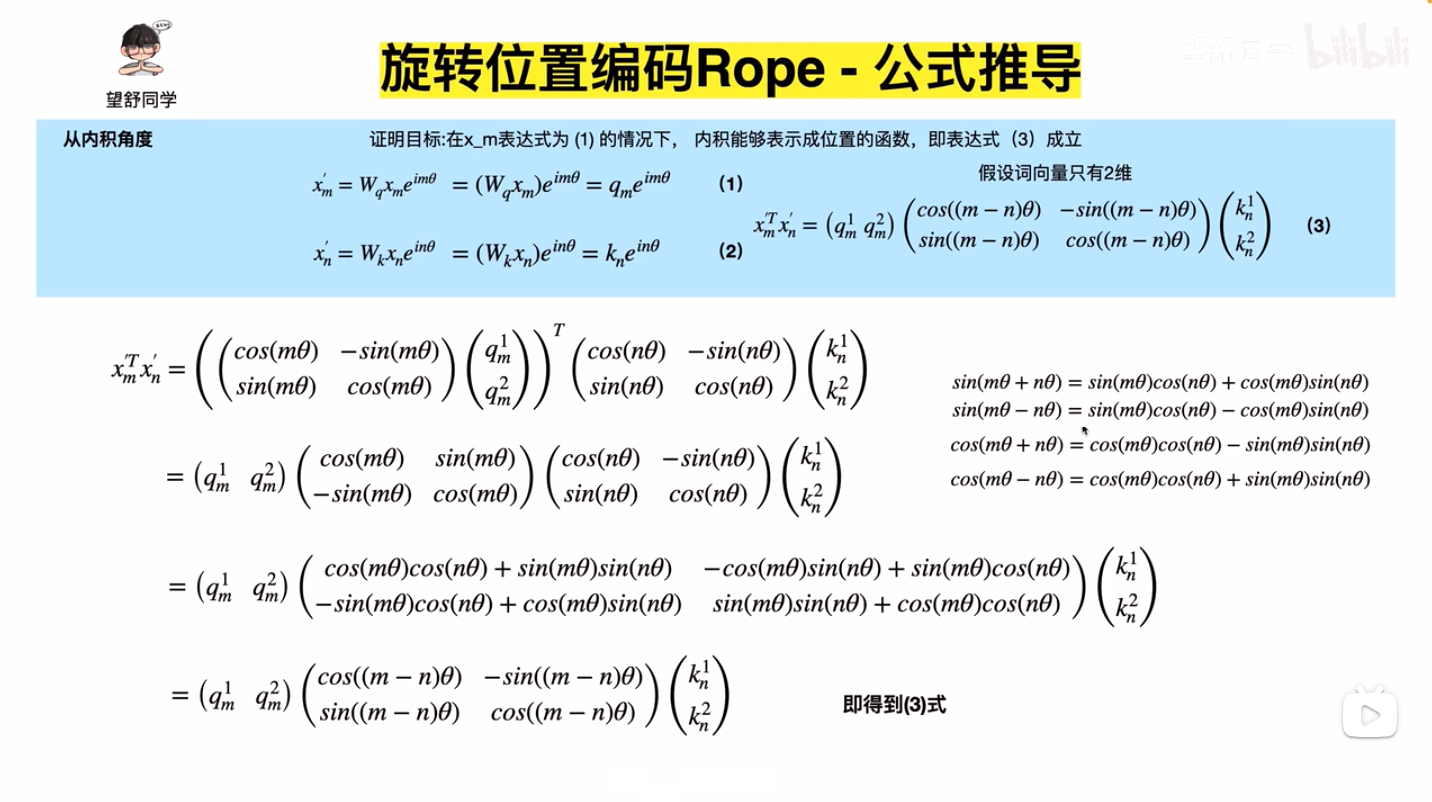
• 公式1,2，推导出公式3的过程（公式角度）
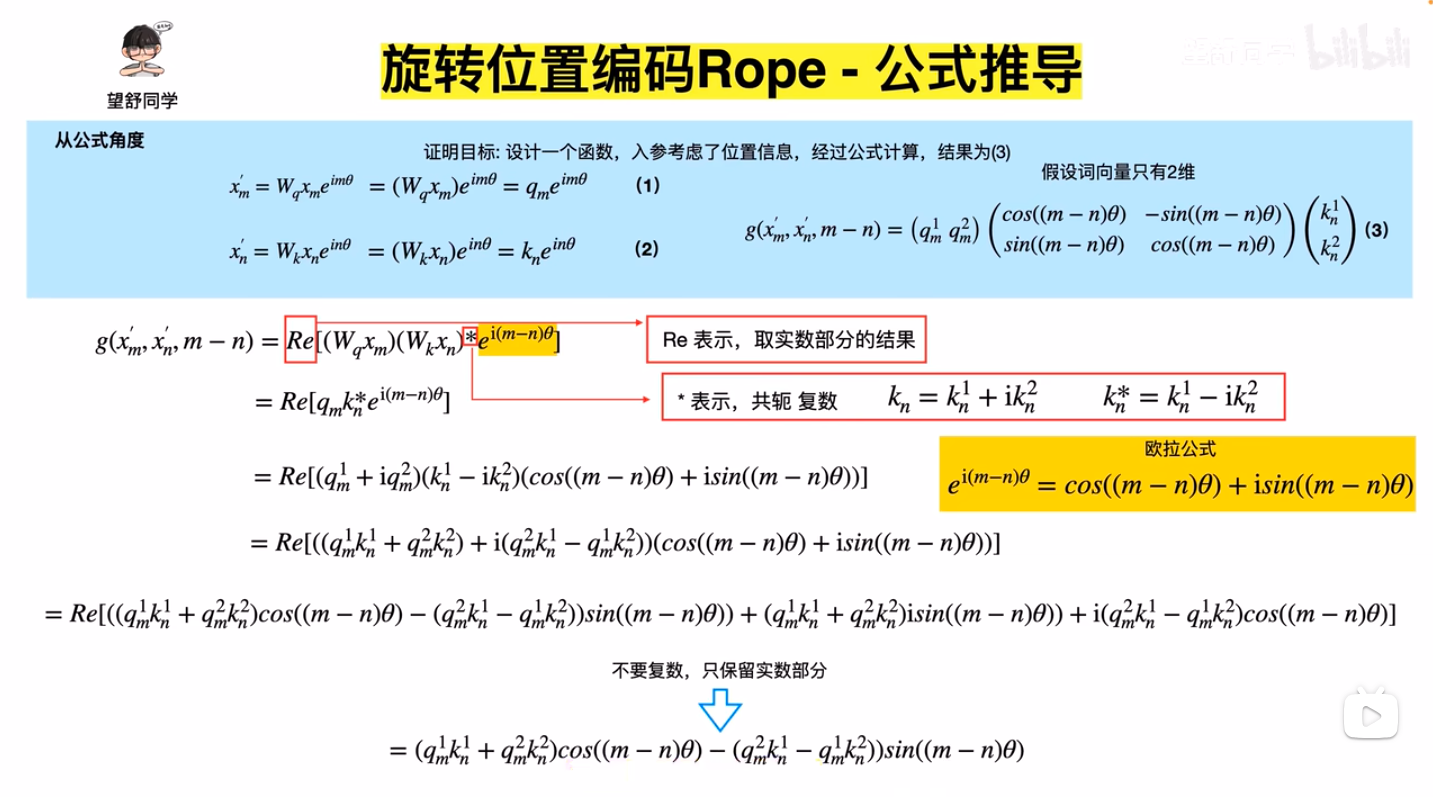
• 内积角度和公式角度推导结果可以对齐
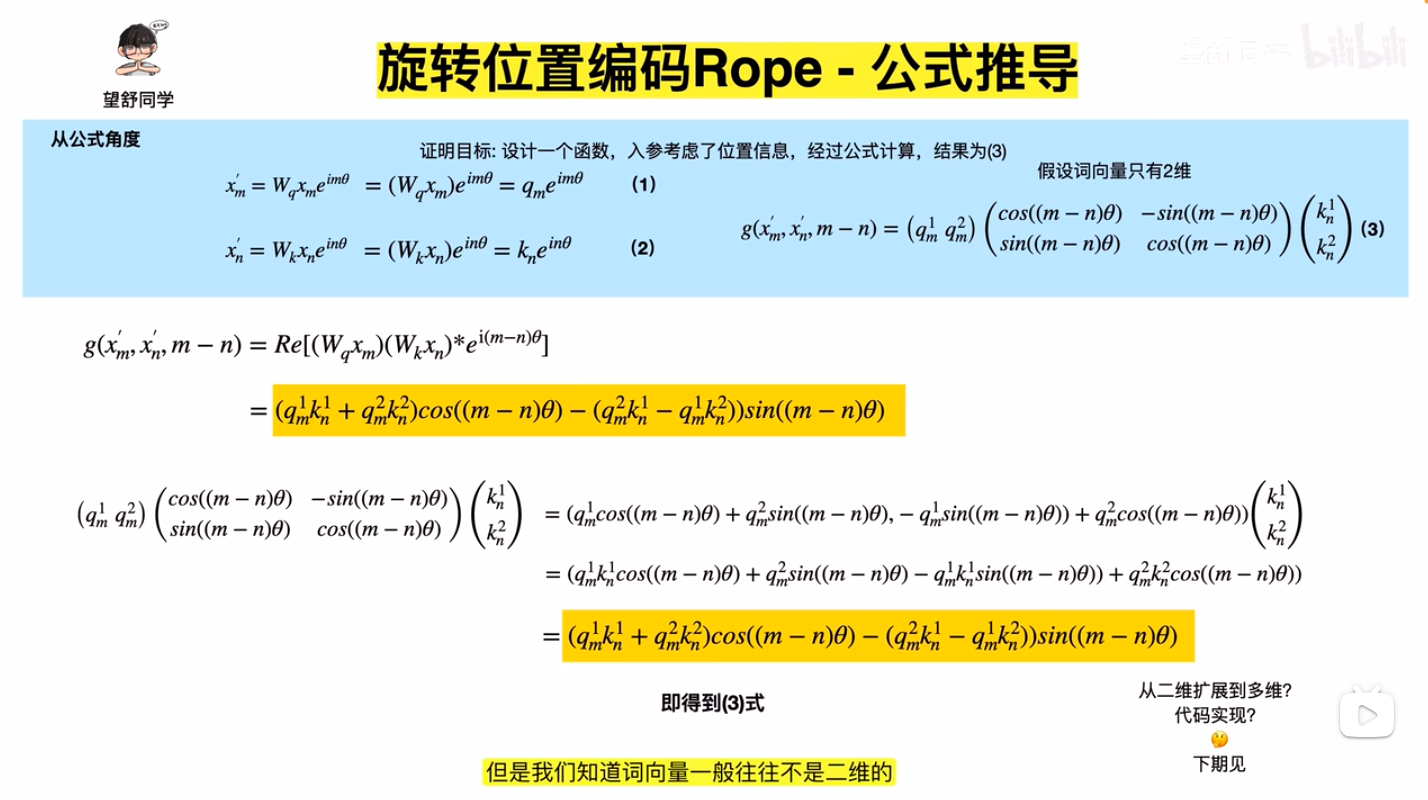
• 扩展到多维的方式，将模型d_model维度按照两两一组分（注意这里不是序列两两分，序列本来做Attention就是两两做内积的），这里要求模型维度是偶数的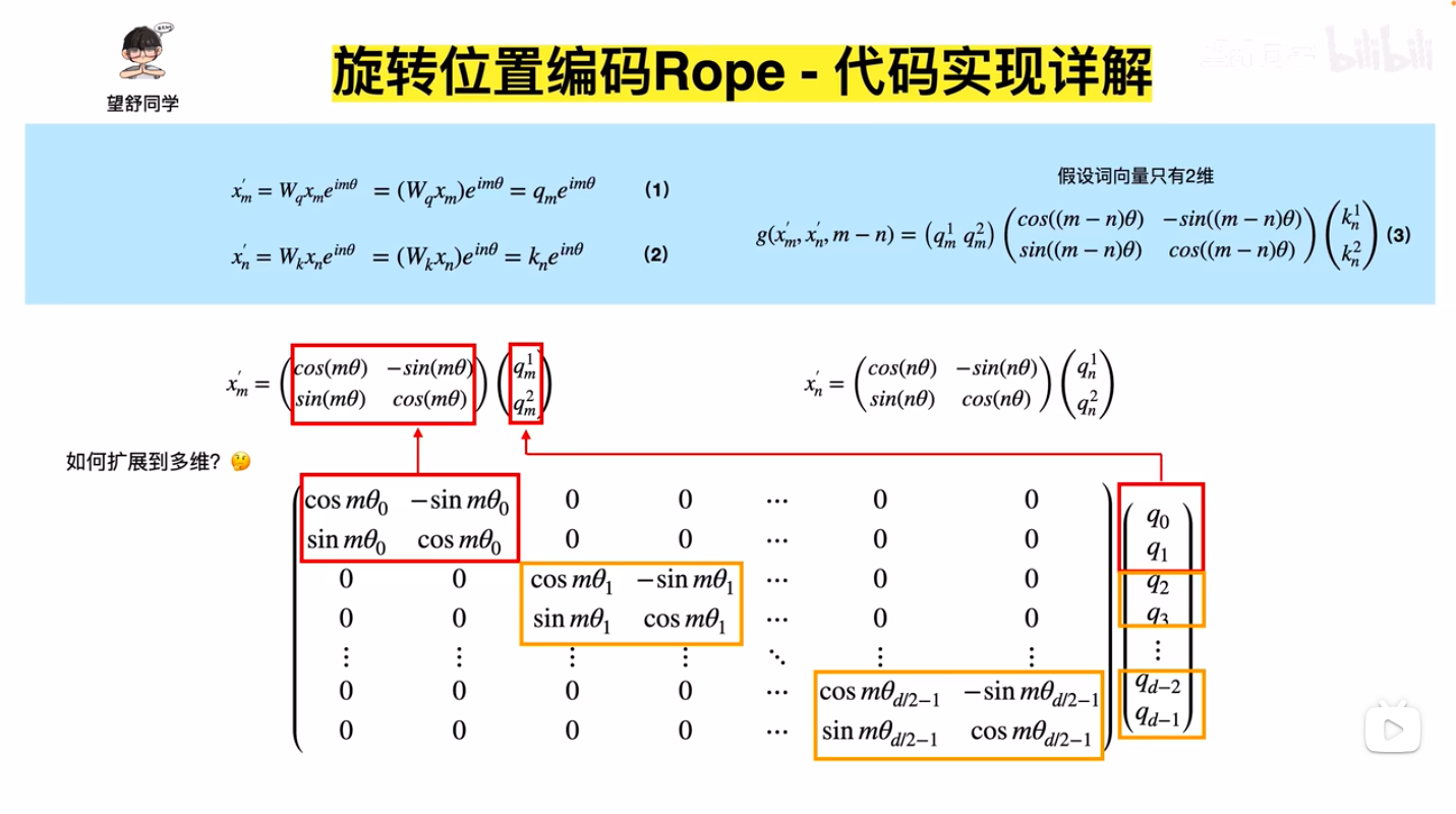
• 公式化简
• 代码实现
  • 上述实现中使用了torch.einsum，本质是爱因斯坦求和约定 ，是矩阵乘法的一种表示，C = torch.einsum("n,d->md", A,B)表示矩阵C[m,d] = A[n]*B[d]，，这是个很常用的省略写法，更详细的可以看看图学 AI：einsum 爱因斯坦求和约定到底是怎么回事？